5 Extracting Road Lengths and Vertices

Ideally, we would want to apply the following approach for each state/UT to get the aggregate road lengths and vertices for all of India:

Get the roads that spatially intersect (approximately) the state/UT
Calculate the min/max/mean/sum lengths and vertices of intersecting roads
Add these calculated values to the admin data

The goal is to have road length and vertex statistics for each state/UT in India for a more numeric comparison between states/UTs, and possibly some more accurate maps. However, we will process only an average sized state in the dataset as the rest of the states/UTs will simply be repetitions of the approach above.

Note 1: The spatial intersection (first step of our approach) here may not be completely accurate as we are only checking for roads that intersect each state/UT, but we are not trimming/cutting long roads that lie inside a state/UT and extend partially outside of it.

Note 2: For simplicity, We have not projected the geographic coordinates (spherical coordinates measured from earth’s center) into planar coordinates (projected geographic coordinates onto a 2D surface) so the intersection algorithm may also not be completely accurate when measuring distances to determine if roads intersect the state/UTs.

5.1 Picking the State/UT for Our Approach

We will look at the different areas of the states/UTs in kilometers squared, and pick a state closest to the average area as our selection criteria. The idea is to select a state with an average area so we have an idea how long it will roughly take to process one state of average size.

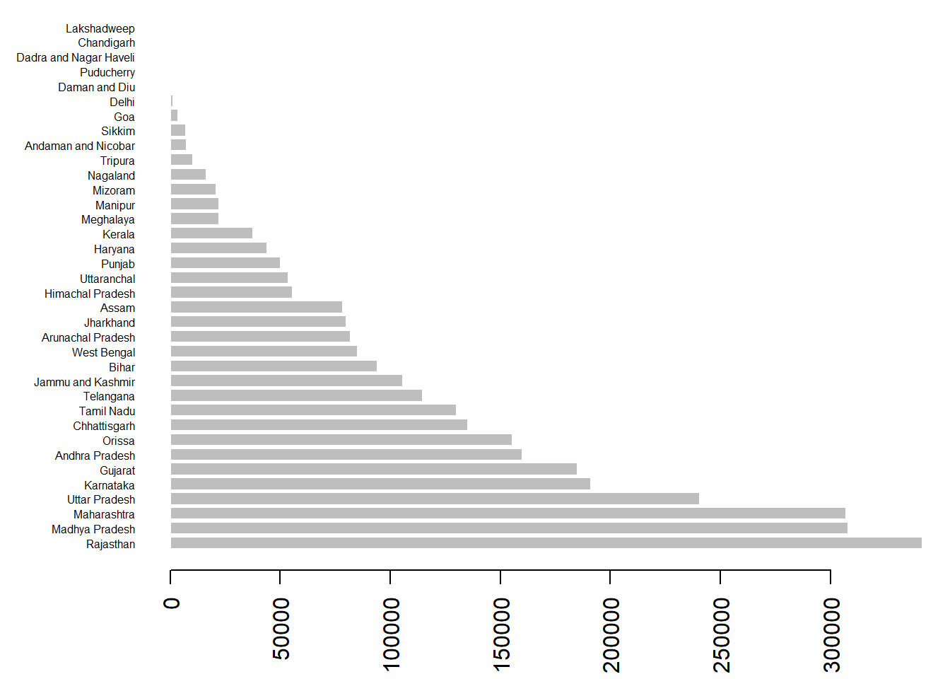
First, we can compute the areas in kilometers squared and add it to our administrative areas data admin, then plot it as a bar graph:

# Get areas in kilometers squared, covert to km squared and add it to the data
admin$area <- st_area(admin)
admin$area <- units::set_units(admin$area, "km^2") # convert to kilometers

# Sort the data by area
admin <- admin[order(-admin$area), ]

# Produce a bar plot of the state/UT names and their areas
x <- as.numeric(admin$area)
y <- admin$NAME_1
options(scipen=5) # Prevent scientific notation for our plot
par(mar=c(4, 6, 0, 1)) # Increase margins to fit plot
barplot(x, names.arg = y,
        horiz = T, las = 2, cex.names = 0.5, # hor. labels
        border = "white") # line color of bars

We can see from the graph that India has relatively even number of state/UTs of varying sizes from 34 kilometers squared to 341902 kilometers squared.

Next, we want to get the state closest to the average size given all states/UTs in India. For reference, this will be the state/UT with an area that has the smallest absolute difference from the average state/UT area:

The mean can be calculated as:

\[ \bar{x} = \frac{x_1 + x_2 + x_3 \dots x_n}{n} \]

where \(\bar{x}\) is the average area of all state/UTs, \(x_1 + x_2 + x_3 \dots x_n\) is the sum of the areas for a states 1 to 36, and \(n\) is the number of states (36 in this case).

x <- admin$area
xMean <- mean(x)

The absolute differences from the average area for each state/UT are then represented as a set \(\{d_1, d_2, d_3 \dots d_n\}\) given by subtracting the state/UT areas \(\{x_1, x_2, x_3, \dots x_n\}\) from the average area of all state/UTs \(\bar{x}\):

\[ \{d_1, d_2, d_3 \dots d_n\} = | \{x_1, x_2, x_3, \dots x_n\} - \bar{x}| \]

d <- abs(x - xMean)

We then want the state/UT with the smallest difference from the set (the state/UT with an area closest to the average size of all states/UTs in India), stored in the variable stateUT:

\[ min(\{d_1, d_2, d_3 \dots d_n\}) \]

dMin <- min(d)
stateUT <- admin[which(d == dMin),]

Let’s inspect the state/UT we picked from our selection criteria:

stateUT[, c("NAME_1", "area")]

## Simple feature collection with 1 feature and 2 fields
## geometry type:  MULTIPOLYGON
## dimension:      XY
## bbox:           xmin: 85.82636 ymin: 21.53945 xmax: 89.87755 ymax: 27.22103
## epsg (SRID):    4326
## proj4string:    +proj=longlat +datum=WGS84 +no_defs
##         NAME_1            area                       geometry
## 36 West Bengal 85229.17 [km^2] MULTIPOLYGON (((88.01861 21...

We can see that we selected state/UT West Bengal, with an area of about 85229 kilometers squared, which is close to the average area of approximately 87565 kilometers squared.

5.2 Extracting Intersecting Roads

Now that we have chosen our state/UT, lets start the extraction by trying to get all the roads that intersect a single state/UT (since this is the start of the process, we also want to keep track of the processing time with Sys.time):

# Track the start time of our extraction process for a single state/UT
startTime1 <- Sys.time()

# Get intersecting roads for state/UT
inStateUT <- st_intersects(roads, stateUT, sparse = F)
stateUTRoads <- roads[inStateUT, ]

# Time for intersection processing
intersectTime <- Sys.time() - startTime1

# Plot the intersecting roads with the state/UT to check
plot(st_geometry(stateUT), axes = T, border = "red")
plot(st_geometry(stateUTRoads), add = T)

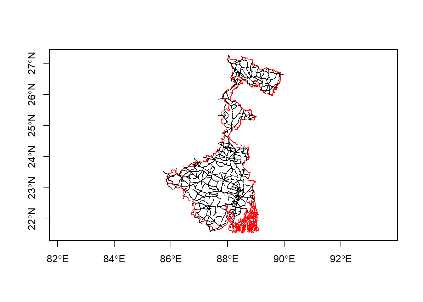
Looking at the plot, we can see that we have extracted the roads that touch or intersect the second state West Bengal, but it does not actually trim or cut the roads when they extend past the state/UT borders. We can use st_intersection (will trim and only keep geometries that are inside the state/UT) for more accuracy, but the computation time would rise, so we will stick with st_intersects (only checks for TRUE or FALSE comparisons, but does not modify the geometries) for the purpose of this walkthrough.

5.3 Calculating Road Lengths and Vertex Statistics

Lets move on and extract the min/max/mean/sum road lengths and vertices for West Bengal:

# Track the time it takes for calculating road lengths and vertices
startTime2 <- Sys.time()

# Extract the length stats
stateUTRoadsLength <- st_length(stateUTRoads)
stateUTLengthStats <- c(min(stateUTRoadsLength, na.rm = T),
                        max(stateUTRoadsLength, na.rm = T),
                        mean(stateUTRoadsLength, na.rm = T),
                        sum(stateUTRoadsLength, na.rm = T))
stateUTLengthStats <- as.numeric(stateUTLengthStats)

# Extract the vertices stats
stateUTRoadsVertex <- npts(stateUTRoads, by_feature = T)
stateUTVertexStats <- c(min(stateUTRoadsVertex, na.rm = T),
                        max(stateUTRoadsVertex, na.rm = T),
                        mean(stateUTRoadsVertex, na.rm = T),
                        sum(stateUTRoadsVertex, na.rm = T))
stateUTVertexStats <- as.numeric(stateUTVertexStats)

# Time for calculating lengths and vertices
calcTime <- Sys.time() - startTime2

# Combine the stats and name them
stateUTStats <- c(stateUTLengthStats, stateUTVertexStats)
names(stateUTStats) <- c("min_length_meters",
                         "max_length_meters",
                         "mean_length_meters",
                         "sum_length_meters",
                         "min_vertices_meters",
                         "max_vertices_meters",
                         "mean_vertices_meters",
                         "sum_vertices_meters")
print(stateUTStats)

##    min_length_meters    max_length_meters   mean_length_meters 
##            0.2127547        73176.4567143        11770.4498551 
##    sum_length_meters  min_vertices_meters  max_vertices_meters 
##     10534552.6203188            2.0000000           57.0000000 
## mean_vertices_meters  sum_vertices_meters 
##            9.2122905         8245.0000000

5.4 Adding Statistics to the State/UT

Finally, we can add the calculated road lengths and vertex statistics to the state/UT West Bengal by converting it into a dataframe, adding the statistics, and then converting it back into a sf object:

# Add the stats to the single state/UT
stateUT <- data.frame(stateUT)
stateUT[, names(stateUTStats)] <- stateUTStats
stateUT <- st_sf(stateUT)

# Interactively view the results
mapview(stateUT, viewer.suppress = F)

Click on the state, and you will now notice that there are extra data on the road length and vertex statistics added to it. If we had done this for all the other states/UTs, we can compare them using numbers, and highlight states/UTs with road densities that are higher than normal to give a better visual representation of our data, but for now we have shown that we can indeed process one state/UT in a reasonable amount of time, and can repeat this process for all the other 35 states/UTs.

5.5 Reviewing the Processing Times for Extraction

Now that we have extracted the road lengths and vertices for the state, we can check how long it took us approximately to process the steps. Remember that we tracked the intersection processing time intersectTime and road length/vertices calculation time calcTime.

Lets have a look at these:

# Calculate the total processing time
totalTime <- intersectTime + calcTime

# Display the processing times
cat("Spatial Intersection:", format(intersectTime, usetz = T),
    "\nRoad Length/Vertices Calculation Time:", format(calcTime, usetz = T),
    "\nTotal Time:", format(totalTime, usetz = T))

## Spatial Intersection: 10.889 secs 
## Road Length/Vertices Calculation Time: 0.04802299 secs 
## Total Time: 10.93702 secs

We can see that the total time for our extraction approach is 10.93702 secs, which could roughly be more or less 10.93702 secs multiplied by 36 (the number of state/UTs) for an estimate of 393.7328 secs. This could scale to much larger processing times if we were to use more detailed data, or if we were to use smaller levels of administrative boundaries/geometries of interest. However, processing one state/UT will give us a good idea of how long it will take to process all states/UTs.

Note: We did not consider the min/max/mean/sum calculations that may factor into the time and the addition of the calculated statistics into the admin dataset, but they generally should not take too much processing time.