Pedalling Forward: The Evolution of Dedicated Cycling Infrastructure in Canadian Cities from 2010 to 2022
R Code for Figures and Tables
Richard Wen richard.wen@utoronto.ca
Konrad Samsel konrad.samsel@mail.utoronto.ca
Brice Batomen brice.kuimi@utoronto.ca
Linda Rothman linda.rothman@torontomu.ca
April 21, 2026
NOTE: Please allow ~30 seconds for the page to load completely.
Installation
For more details, see Software and Package Versions.
Running This Code
- Ensure the installation steps above are completed
- Download a zip of the code and data here
and unzip it
- Code Repository: github.com/rrwen/recovr-infracycle
- In RStudio, open the src/src.Rproj file
- Then, open the src/index.Rmd file
- In RStudio:
- Run all code: Click the
Rundrop down (top right of the code pane) and clickRun All - Generate HTML version: Click
knit(top left of code pane) and a file will be generated indocs/index.html(you may have to try a couple times to succeed due towebshot2timeouts)
- Run all code: Click the
Libraries
Install R packages if needed.
# Required packages
required_packages <- c(
"rmarkdown",
"bookdown",
"knitr",
"tidyverse",
"glue",
"readxl",
"ggtext",
"scales",
"patchwork",
"DiagrammeR",
"DiagrammeRsvg",
"webshot2",
"magick",
"rsvg",
"sf",
"tmap",
"ggspatial",
"prettymapr",
"units",
"lubridate",
"kableExtra",
"DT",
"binom",
"boot",
"R.devices"
)
# Try to install packages if not installed
default_options <- options()
tryCatch(
{
# Disable interactivity
options(install.packages.compile.from.source = "always")
# Install package if not installed
for (package in required_packages) {
is_package_installed <- require(package, character.only = TRUE)
if (!is_package_installed & package != "osmplotr") {
cat(paste0("Installing package: ", package, "\n"))
install.packages(package)
} else {
cat(paste0("Package already installed: ", package, "\n"))
}
}
},
error = function(cond) {
stop(cond)
},
finally = {
options(default_options) # reset interactivity
}
)Load R libraries.
Settings
settings <- list()
# Infrastructure types in order
settings$type_recode_infra <- c(
PBL = "Cycle Track",
BUF = "Buffered Lane",
PL = "Painted Lane",
LSB = "Local Street\nBikeway"
)
# Infrastructure types to remove
settings$type_filter_infra <- c("N", "None", "SR")
# Road types in order
settings$type_recode_road <- c(
Arterial = "Arterial",
Collector = "Collector",
Local = "Local"
)
# Column references
settings$year_col_road <- "verify_install_year"
settings$type_col_road <- "road_type_recode"
settings$type_col_infra <- "verify_install_type"
# Set years of interest
settings$year_min <- 2009
settings$year_max <- 2022
# Plot settings
settings$line_year <- 2019
settings$basemaps <- c(
"CartoDB.Positron",
"CartoDB.DarkMatter",
"Esri.WorldGrayCanvas"
)
# Map infrastructure changes since year
settings$infra_changes_year <- 2020
# Apply map settings
tmap_options(basemaps = settings$basemaps)Functions
Function A: ggsave
Workaround to fix ggsave not working with RmD run
command in RStudio.
Also skips saving as a default. ggsave seems to be
causing this markdown document to error out. Running each
ggsave repeatedly, eventually results in success.
If figures need to be regenerated, simply modify argument
skip to FALSE.
Function 0: datatable
Modify the default datatable function from
DT library to generate interactive tables:
datatable <- function(...) {
# Build arg list
args <- list(...)
# Default custom filename
filename <- if (!"filename" %in% names(args)) "data" else args$filename
args[["filename"]] <- NULL
# Add default extensions
args$extensions <- if (!"extensions" %in% names(args)) "Buttons" else args$extensions
# Add default args
args$filter <- if (!"filter" %in% names(args)) "top" else args$filter
args$fillContainer <- if (!"fillContainer" %in% names(args)) T else args$fillContainer
# Add default options
if (!"options" %in% names(args)) {
args$options <- list(
scrollY = "350px",
buttons = list(
list(
extend = "csv",
filename = filename,
exportOptions = list(columns = ":not(.rownames)")
),
list(
extend = "excel",
filename = filename,
exportOptions = list(columns = ":not(.rownames)"),
title = ""
)
),
columnDefs = list(
list(
targets = 0,
className = "rownames"
)
),
dom = "Bfrtip"
)
}
return(do.call(DT::datatable, args))
}Function 1: calc_yearly_len
Calculate yearly road lengths.
The following function calculates yearly road lengths by infrastructure type using cumulative sums and filling in missing years and types.
For a given infrastructure type, the total road length for a given year is expressed below:
\[ length_{year,type} = f(year,type) = \sum_{i=year_{min}}^{year}l_{i, type}\ \mid\ l_{i, type} \geq 0 \]
Where:
- \(year\) is the given year
- \(type\) is the infrastructure type
- \(year_{min}\) is the earliest year available in the data
- \(l_{i,type}\) is the road length \(l\) for previous years \(i\) and infrastructure \(j\)
- \(l_{i,type}\) is set to 0 if there is no data
#' Calculate Yearly Road Lengths By Infrastructure Type
#'
#' Calculates the cumulative yearly road lengths by infrastructure type without considering infrastructure changes.
#'
#' @param df A data.frame with three columns containing the year, type, and road lengths.
#' @param year_col The name (char) or index (int) of the column containing the years.
#' @param type_col The name (char) or index (int) of the column containing the infrastructure type
#' @param len_col The name (char) or index (int) of the column containing the road lengths.
#' @param out_col The name (char) of the column containing the calculated yearly road lengths by type.
#'
#' @return A data.frame with three columns containing the year, type, and calculated yearly road lengths by type.
#' @export
#'
calc_yearly_len <- function(
df,
year_col = "verify_install_year",
type_col = "verify_install_type",
len_col = "geometry_len_km",
out_col = "len",
year_min = settings$year_min,
year_max = settings$year_max
) {
# Convert data types
df <- as.data.frame(df)
df[[year_col]] <- as.integer(df[[year_col]])
df[[type_col]] <- as.character(df[[type_col]])
df[[len_col]] <- as.numeric(df[[len_col]])
# Remove rows with empty type
out <- df %>% filter(
!is.na(.data[[type_col]])
)
# Filter to min and max years
if (year_min > 0) {
df <- df %>% filter(
.data[[year_col]] >= year_min
)
} else {
year_min <- min(out[[year_col]], na.rm = TRUE)
}
if (year_max > 0) {
df <- df %>% filter(
.data[[year_col]] <= year_max
)
} else {
year_max <- max(out[[year_col]], na.rm = TRUE)
}
# Add dummy len for each type and year combo
# Covers cases where type and year combo does not exist
# E.g. No new PL installs in 2021, hence a record PL in 2021 does not exist
type_uniq <- unique(out[[type_col]])
type_n <- length(type_uniq)
year_uniq <- year_min:year_max
year_n <- length(year_uniq)
out <- out %>% add_row(
!!year_col := rep(year_uniq, each = type_n),
!!type_col := rep(type_uniq, year_n),
!!len_col := rep(0, type_n * year_n)
)
# Calc cumsum for each non-empty type ordered by year
out <- out %>%
arrange(.data[[year_col]]) %>%
group_by(.data[[type_col]]) %>%
mutate(
!!out_col := cumsum(.data[[len_col]])
)
# Get the last cumsum for each year and type
out <- out %>%
group_by(.data[[year_col]], .data[[type_col]]) %>%
arrange(desc(row_number())) %>%
slice(1)
# Return only the columns spec
out <- out %>% select(c(
year_col,
type_col,
out_col
))
return(out)
}Function 2: calc_yearly_adj_len
Calculate yearly adjusted road length.
The following function calculates yearly adjusted road lengths by infrastructure type using cumulative sums and filling in missing years and types.
For a given infrastructure type, the total adjusted road length for a given year is expressed below:
\[ length_{year,type}^{install} + length_{year,type}^{change_i} - length_{year,type}^{replacement_i} \]
Where:
- \(length_{year,type}^{install}\) are the yearly cumulative road lengths for an infrastructure \(type\) installation
- \(length_{year,type}^{change_i}\) are the yearly cumulative road lengths for an infrastructure \(type\) change in order \(i\)
- \(length_{year,type}^{replacement_i}\) are the yearly cumulative road lengths for an infrastructure \(type\) replaced by change in order \(i\)
#' Calculate Yearly Adjusted Road Lengths By Infrastructure Type
#'
#' Calculates the cumulative yearly adjusted road lengths by infrastructure type accounting for installations and subsequent changes.
#'
#' @param df A data.frame with three columns containing the year, type, and road lengths.
#'
#' @return A data.frame with columns containing the year, type, cumulative road lengths of installations, changes, and replacements, and calculated yearly adjusted road lengths by type.
#' @export
#'
calc_yearly_adj_len <- function(df, ...) {
# Vars for ref
year_cols <- c("verify_install_year", "verify_upgrade1_year", "verify_upgrade2_year")
type_cols <- c("verify_install_type", "verify_upgrade1_type", "verify_upgrade2_type")
type_col <- "type"
len_col <- "geometry_len_km"
out_col <- "adj_len"
id_col <- "id"
# Ensure df
df <- as.data.frame(df)
# Pivot to long format to capture states per segment
df_long <- df %>%
as.data.frame() %>%
select(all_of(c(
id_col,
type_cols,
year_cols,
len_col
))) %>%
pivot_longer(
cols = all_of(type_cols),
names_to = "stage",
values_to = "type"
) %>%
filter(!is.na(type)) %>%
mutate(
year = case_when(
stage == "verify_install_type" ~ verify_install_year,
stage == "verify_upgrade1_type" ~ verify_upgrade1_year,
stage == "verify_upgrade2_type" ~ verify_upgrade2_year,
.default = NA_real_
)
)
# Create df to capture all yearly states for each segment
df_allstates <- crossing(
id = unique(df_long$id),
year = seq(min(df_long$year), max(df_long$year))
) %>%
left_join(
df_long,
by = c("id", "year")
) %>%
arrange(id, year) %>%
group_by(id) %>%
fill(type, .direction = "down") %>%
fill(geometry_len_km, .direction = "down") %>%
ungroup
# Calc adjusted lengths per year
df_ylens <- df_allstates %>%
group_by(year, type) %>%
filter(!is.na(type)) %>%
summarize(adj_len = sum(geometry_len_km)) %>%
ungroup
# Add zero lens for types not existing in years for plot lines
out <- df_ylens %>%
right_join( # add years for types not existing
crossing(
year = seq(min(df_ylens$year), max(df_ylens$year)),
type = unique(df_ylens$type)
), by = c("year", "type")
) %>%
mutate(
adj_len = if_else(is.na(adj_len), 0, adj_len),
verify_install_type = type
)
return(out)
}Function 3: plot_yearly_len
Plot road lengths by generic types.
This function plots an area chart showing the cumulative road lengths by a user-defined type for each year.
This is a generic function for user-defined types such as infrastructure or road types.
#' Plot Yearly Road Lengths By Type
#'
#' Creates an area plot of road lengths by category types.
#'
#' @param df A data.frame with three columns containing the year, type, and road lengths.
#' @param title The title (char) of the plot.
#' @param title_underline Set to TRUE to underline the title.
#' @param x_title The title (char) of the x-axis.
#' @param y_title The title (char) of the y-axis.
#' @param y_suffix The suffix (char) to add to the end of y axis values.
#' @param y_lim Minimum and maximum road length (numeric) as a vector of length 2 to limit the range of the y-axis. Set to `NULL` for auto.
#' @param legend_title The title (char) of the legend.
#' @param legend Set to TRUE to include a legend.
#' @param year_col The name (char) or index (int) of the column containing the years.
#' @param year_min The minimum year (int) to display.
#' @param year_max The maximum year (int) to display.
#' @param year_int The year intervals (int) to display. For example, 1 displays every year, and 2 displays every two years.
#' @param len_col The name (char) or index (int) of the column containing the road lengths.
#' @param len_per_start Set to `TRUE` to add final percentages at the starting year or `FALSE` to omit this.
#' @param len_per_end Set to `TRUE` to add final percentages at the ending year or `FALSE` to omit this.
#' @param type_col The name (char) or index (int) of the column containing the type.
#' @param type_filter A vector (char) of types to remove fomr the plot.
#' @param type_recode A named vector (char) of names representing types and values representing the values to replace each type with.
#' @param line_km The km (numeric) of the red reference line.
#' @param line_show Set to TRUE to draw the km red reference line.
#' @param line_year Set to a year (int) to draw a reference line for a year. If FALSE, a line will not be drawn.
#' @param color_low The bottom color (char) of the type.
#' @param color_high The top color (char) of the type.
#' @param color_manual A set of manual colors to use for the areas. The default `NULL` uses `color_low` and `color_high` instead.
#' @return An area ggplot of the cumulative yearly road lengths by type.
#' @export
#'
plot_yearly_len <- function(
df,
title = "",
title_underline = TRUE,
x_title = "",
y_title = "",
y_suffix = " km",
y_lim = NULL,
legend_title = "Type",
legend = TRUE,
year_col = "year",
year_min = FALSE,
year_max = FALSE,
year_int = 1,
len_col = "adj_len",
len_per_start = FALSE,
len_per_end = FALSE,
type_col = "type",
type_filter = c(),
type_recode = c(),
line_km = 10,
line_show = FALSE,
line_year = FALSE,
color_low = "#DFEBF7",
color_high = "#3683BB",
color_manual = NULL
) {
# Filter to start and end years
if (year_min > 0) {
df <- df %>% filter(
.data[[year_col]] >= year_min
)
}
if (year_max > 0) {
df <- df %>% filter(
.data[[year_col]] <= year_max
)
}
# Filter out particular infrastructure types
if (length(type_filter) > 0) {
df <- df %>% filter(
!.data[[type_col]] %in% type_filter
)
}
# Recode and reorder category types
if (length(type_recode) > 0) {
# Reorder category types
type_uniq <- unique(df[[type_col]])
type_reorder <- names(type_recode)
type_reorder <- c(type_reorder, type_uniq[!type_uniq %in% type_reorder])
df[[type_col]] <- factor(df[[type_col]], levels = type_reorder)
# Recode category types
df[[type_col]] <- recode(df[[type_col]], !!!type_recode)
}
# Create fill colors
type_n <- length(type_uniq)
if (is.null(color_manual)) {
type_colors <- scales::seq_gradient_pal(
color_low,
color_high
)(seq(0, 1, length.out = type_n))
} else {
type_colors <- color_manual
}
# Create base area plot with legend and labels
len_max <- max(df[[len_col]], na.rm = TRUE)
year_max <- max(df[[year_col]], na.rm = TRUE)
out <- ggplot(
df,
aes(
x = .data[[year_col]],
y = .data[[len_col]],
fill = .data[[type_col]],
order = desc(.data[[type_col]])
)
) +
geom_area(colour = NA, alpha = 0.7) +
scale_fill_manual(values = type_colors) +
geom_line(
position = "stack",
size = 0.2
) +
labs(
x = x_title,
y = y_title,
fill = legend_title
) +
guides(
fill = FALSE,
color = FALSE
) +
scale_x_continuous(
breaks = seq(year_min, year_max, by = year_int),
labels = seq(year_min, year_max, by = year_int),
limits = c(if (len_per_start) year_min - 1 else year_min, if (len_per_end) year_max + 1 else year_max)
) +
scale_y_continuous(
label = scales::label_number(suffix = y_suffix)
) +
theme_minimal() +
theme(
plot.margin = unit(c(5,5,5,5), "points")
)
# Scale road length axis y
if (!is.null(y_lim)) {
out <- out + ylim(y_lim)
}
# Add title
if (title_underline) {
out <- out + ggtitle(
bquote(underline(.(title)))
)
} else {
out <- out + ggtitle(title)
}
# Add legend
if (legend) {
out <- out + guides(fill = guide_legend(
reverse = FALSE,
override.aes = list(
alpha = 0.7,
color = NA,
shape = NA
)
))
}
# Add percentages to start
if (len_per_start) {
df_perc_start <- df %>% filter(
.data[[year_col]] == year_min
) %>% arrange(desc(.data[[type_col]])) %>% mutate(
len = cumsum(.data[[len_col]]) - (.data[[len_col]] / 2),
perc = .data[[len_col]] / sum(.data[[len_col]], na.rm = T)
) %>% filter(
perc > 0
) %>% mutate(
perc = paste0(round(perc * 100, 1), "%")
)
out <- out + geom_text(
data = df_perc_start,
x = year_min,
size = 2.75,
hjust = 1.225,
aes(
y = len,
label = perc
)
)
}
# Add percentages to end
if (len_per_end) {
df_perc_end <- df %>% filter(
.data[[year_col]] == year_max
) %>% arrange(desc(.data[[type_col]])) %>% mutate(
len = cumsum(.data[[len_col]]) - (.data[[len_col]] / 2),
perc = .data[[len_col]] / sum(.data[[len_col]], na.rm = T),
) %>% filter(
perc > 0
) %>% mutate(
perc = paste0(round(perc * 100, 1), "%")
)
out <- out + geom_text(
data = df_perc_end,
x = year_max,
size = 2.75,
hjust = -0.225,
aes(
y = len,
label = perc
)
)
}
# Add dotted year ref line
if (line_year) {
out <- out + geom_vline(
xintercept = line_year,
color = "black",
linetype = "dashed"
)
}
# Add red 50km ref line
if (line_show) {
out <- out + geom_segment( # 50km red line
aes(
x = 2009,
y = 0,
xend = 2009,
yend = line_km,
color = "#bb0000"
)
) +
geom_segment( # 50km red triangle point down
aes(
x = 2009,
y = (line_km + 0.01) - (len_max * 0.05),
xend = 2009,
yend = line_km - (len_max * 0.05),
color = "#bb0000"
),
arrow = arrow(
length = unit(0.03, "npc"),
ends = "last",
type = "closed"
)
) +
geom_segment( # 50km red triangle point up
aes(
x = 2009,
y = (len_max * 0.05) - 0.01,
xend = 2009,
yend = (len_max * 0.05),
color = "#bb0000"
),
arrow = arrow(
length = unit(0.03, "npc"),
ends = "last",
type = "closed"
)
) +
annotate(
"text",
x = 2009,
y = line_km,
label = paste0(line_km, "km"),
color = "#bb0000",
hjust = -0.225
)
}
return(out)
}Function 3a: plot_yearly_len_infra
Plot yearly adjusted road lengths by infrastructure type.
This function plots area charts of yearly road lengths by infrastructure types for a list of data.
This uses the plot_yearly_len function.
#' Plot Yearly Road Lengths By Infrastructure Type
#'
#' Creates area plots of road lengths by infrastructure type.
#'
#' @param df_list A list of lists, where each key is the title and each value contains a list with the following structure:
#' \itemize{
#' \item \code{data}: data.frame containing the install and change years, type, and road segment lengths.
#' \item \code{roadway_total}: the total roadway length if `rodway_per` is given. This is used as the denominator to normalize road lengths.
#' \item \code{roadway_per}: Number of units of total roadway length (numeric) to normalize by (e.g. 1000 means per 1000 km of roadway). Set to `NULL` or omit to disable normalization of road lengths.
#' \item \code{color_manual}: Optional color of the area polygons to be set manually.
#' }
#' @param len_title The title (char) for the road lengths.
#' @param line_show Set to `TRUE` to add a 50km reference line.
#' @param ... Additional arguments passed to `plot_yearly_len`.
#'
#' @return Multiple area ggplots of the cumulative yearly road lengths by infrastructure type combined with patchwork.
#' @export
#'
plot_yearly_len_infra <- function(
df_list,
len_title = "Total length per 1000 centreline-km of roadway",
line_km = 10,
line_show = TRUE,
...
) {
# Create infra plots from data
p <- list()
pdata <- list()
for (i in 1:length(df_list)) {
# Get data and plot title
df <- df_list[[i]]$data
ptitle <- names(df_list)[[i]]
# Get roadway vars if exists
roadway_per <- NULL
roadway_total <- NULL
if ("roadway_per" %in% names(df_list[[i]])) {
roadway_per <- df_list[[i]]$roadway_per
}
if ("roadway_total" %in% names(df_list[[i]])) {
roadway_total <- df_list[[i]]$roadway_total
}
# Pivot to long format to capture states per segment
p[[i]] <- calc_yearly_adj_len(df)
# Norm len if needed
len_col <- "adj_len"
if (!is.null(roadway_per)) {
p[[i]] <- p[[i]] %>% mutate(
adj_len_norm =
(adj_len / roadway_total) * roadway_per
)
len_col = "adj_len_norm"
}
# Add infra data
pdata[[i]] <- p[[i]] %>%
mutate(title = ptitle) %>%
select(
title,
year,
adj_len,
adj_len_norm,
everything()
)
# Add infra plot
p[[i]] <- pdata[[i]] %>% plot_yearly_len(
title = ptitle,
year_min = settings$year_min,
year_max = settings$year_max,
type_col = settings$type_col_infra,
type_filter = settings$type_filter_infra,
type_recode = settings$type_recode_infra,
legend_title = "Infrastructure Type",
line_km = line_km,
line_show = line_show,
line_year = settings$line_year,
len_col = len_col,
color_manual = df_list[[i]]$color_manual,
...
)
}
# Y-axis title
y_title <- ggplot() +
annotate(
geom = "text",
x = 1,
y = 1,
label = len_title,
angle = 90,
size = 5
) +
coord_cartesian(clip = "off")+
theme_void()
# Combine all infra plots together
out <- list()
out$data <- pdata %>% bind_rows
out$plot <- (y_title | wrap_plots(p, nrow = length(p))) +
plot_annotation(
title = "Roadways with Dedicated Cycling Infrastructure",
caption = sprintf("Years (%s-%s)", settings$year_min, settings$year_max),
theme = theme(
plot.title = element_text(hjust = 0.5, size = 16),
plot.caption = element_text(hjust = 0.5, size = 14)
)
) +
plot_layout(widths = c(0.05, 1))
return(out)
}Function 3b: plot_yearly_len_road
Plots yearly adjusted road lengths for road types.
This function plots area charts of yearly road lengths by overall road type and by infrastructure separated by each road type.
This uses the plot_yearly_len function.
#' Plot Yearly Road Lengths By Road Type
#'
#' Creates area plots of road lengths by overall road type, and by infrastructure per road type.
#'
#' @param df The data.frame containing the install and change years, type, and road segment types and lengths.
#' @return Multiple area ggplots of the cumulative yearly road lengths by road type combined with patchwork.
#' @export
#'
plot_yearly_len_road <- function(df, title = "Roadways with Dedicated Cycling Infrastructure") {
# Create list to store plots and data
p <- list()
pdata <- list()
# Format plot data
pdata[[1]] <- calc_yearly_len(
df,
year_col = settings$year_col_road,
type_col = settings$type_col_road
) %>% mutate(
road_type = "All"
)
# Plot overall road types
p[[1]] <- pdata[[1]] %>%
plot_yearly_len(
title = title,
title_underline = FALSE,
year_col = settings$year_col_road,
year_min = settings$year_min,
year_max = settings$year_max,
x_title = sprintf("Years (%s-%s)", settings$year_min, settings$year_max),
y_title = "Total Length (Centreline km)",
legend_title = "Roadway Type",
type_col = settings$type_col_road,
type_recode = settings$type_recode_road,
len_col = "len",
line_show = FALSE,
line_year = settings$line_year,
color_low = "#C1DDB3",
color_high = "#297A22"
) +
theme(
plot.title = element_text(size = 18),
plot.margin = margin(0, 0, 0, 0, "pt")
)
# Plot arterial, collector, and local road by infra
rtypes <- c("Arterial", "Collector", "Local")
for (i in 1:length(rtypes)) {
# Get road type
r <- rtypes[i]
# Format infra data for road type
pdata[[i + 1]] <- calc_yearly_adj_len(
df %>% filter(.data[[settings$type_col_road]] == r),
type_col = settings$type_col_infra
) %>%
mutate(
road_type = r
)
# Create infra plot for road type
p[[i + 1]] <- pdata[[i + 1]] %>%
plot_yearly_len(
title = sprintf("%s Roadways", r),
title_underline = FALSE,
line_show = FALSE,
line_year = settings$line_year,
year_int = 2,
x_title = sprintf("Years (%s-%s)", settings$year_min, settings$year_max),
y_title = "Total Length (Centreline km)",
year_min = settings$year_min,
year_max = settings$year_max,
type_col = settings$type_col_infra,
type_filter = settings$type_filter_infra,
type_recode = settings$type_recode_infra,
legend_title = "Infrastructure Type"
) +
theme(
plot.title = element_text(size = 14),
plot.margin = margin(0, 12, 0, 0, "pt")
)
}
# Plot horizontal gradient bar
grad_bar <- ggplot(data.frame(x = 1:4), aes(x = x, y = 1, color = x)) +
geom_line(size = 4) +
scale_color_gradient(low = "#C1DDB3", high = "#297A22") +
theme_void() +
guides(color = FALSE) +
theme(
axis.title = element_blank(),
axis.text = element_blank(),
axis.ticks = element_blank(),
axis.line = element_blank(),
plot.margin = margin(0, 0, 0, 0, "pt")
)
# Plot overall and road type plots together
out <- list()
out$data <- pdata %>%
bind_rows %>%
select(
road_type,
year,
verify_install_year,
len,
adj_len,
everything()
)
out$plot <- ( # overall plot
plot_spacer() +
p[[1]] +
plot_spacer() +
plot_layout(
widths = c(0.25, 0.35, 0.2)
)
) / ( # gradient bar
plot_spacer() +
grad_bar +
plot_spacer() +
plot_layout(widths = c(-0.8, 10, -1.1))
) / ( # infra plots
p[[2]] +
p[[3]] +
p[[4]]
) + plot_layout(
heights = c(12, 1, 8)
) + plot_annotation( # A B tags
tag_levels = list(c("A", "", "B", "", ""))
) & theme(
plot.tag = element_text(face = "bold", size = 12)
)
return(out)
}Function 4: plot_yearly_diff
Plots differences between two years.
This function plots a bar chart of differences between two columns containing years.
This function is used to check the differences in installation years between the city’s data and the verified data.
#' Plot Yearly Differences
#'
#' Creates a bar plot of the differences between two years.
#'
#' @param df The data.frame containing the two columns with the years.
#' @param year_col1 The name (char) or index (int) of the first year column.
#' @param year_col2 The name (char) or index (int) of the second year column to be subtracted from.
#' @param year_col1_name The name alias (char) of the first year column year_col1.
#' @param year_col2_name The name alias (char) of the second year column year_col2.
#' @param year_min The minimum year (int) to calculate differences for.
#' @param year_max The maximum year (int) to calculate differences for.
#' @param title The title (char) of the plot.
#' @param title_n Set to TRUE to add the number of total segments considered.
#' @param x_title The title (char) of the x-axis.
#' @param y_title The title (char) of the y-axis.
#' @param x_breaks The number (int) of breaks to show on the x-axis. Set to FALSE to let ggplot automatically decide.
#' @param x_lim A vector of size two specifying the limits of the x-axis. Set to FALSE to skip.
#' @param x_perc Set to TRUE to show proportions and FALSE to show counts.
#' @param out_data Set to TRUE to return a list
#'
#' @return A ggplot of yearly differences (year_col2 - year_col1), displaying the proportion of rows for each difference in years. If `out_data` is TRUE then returns a list with keys `data` representing the data used for plotting and `plot` with the ggplot object.
#' @export
#'
plot_yearly_diff <- function(
df,
year_col1 = "install_year",
year_col2 = "verify_install_year",
year_col1_name = "City Year",
year_col2_name = "Verified Year",
year_min = settings$year_min,
year_max = settings$year_max,
title = sprintf(
"Difference in Years, Comparing %s and %s",
year_col1_name,
year_col2_name
),
title_n = TRUE,
x_title = sprintf(
"Difference in Years (%s - %s)",
year_col2_name,
year_col1_name
),
y_title = "Proportion of Total Segments",
x_breaks = 15,
x_lim = FALSE,
x_perc = TRUE,
out_data = TRUE
) {
# Filter for comparable rows only
pdata <- df %>% filter(
!is.na(.data[[year_col1]]) & !is.na(.data[[year_col2]])
)
# Filter within min year
if (year_min) {
pdata <- pdata %>% filter(
.data[[year_col2]] > year_min
)
}
# Filter within max year
if (year_max) {
pdata <- pdata %>% filter(
.data[[year_col2]] <= year_max
)
}
# Add n to title
if (title_n) {
title <- sprintf("%s (n=%s)", title, nrow(pdata))
}
# Calc yearly diff
pdata <- pdata %>%
mutate(year_diff = .data[[year_col2]] - .data[[year_col1]]) %>%
count(year_diff) %>%
mutate(n_perc = (n / sum(n)) * 100)
# Set to proportions or counts
pdata$y <- if (x_perc) pdata$n_perc else pdata$n
# Plot yealy diffs
out <- pdata %>%
ggplot(aes(
x = year_diff,
y = y
)) +
geom_bar(
stat = "identity",
color = "#332a94",
fill = "#c3d5e4",
width = 1
) +
labs(
title = title,
x = x_title,
y = y_title
) +
theme(
plot.title = element_text(size = 12)
)
# Add percentage sign if percentages
if (x_perc) {
out <- out +
scale_y_continuous(
label = scales::label_number(suffix = "%")
)
}
# Set x interval breaks
if (x_breaks) {
out <- out + scale_x_continuous(
breaks = scales::breaks_pretty(x_breaks)
)
}
# Set x limits
if (length(x_lim) > 1) {
out <- out + coord_cartesian(xlim = x_lim)
}
# Returns ggplot obj or list
if (out_data) {
out <- list(
data = pdata %>% as_tibble %>% select(-geometry, -y),
plot = out
)
}
return(out)
}Function 5: filter_criteria
Filter for segment inclusion criteria.
This function applies segment inclusion critieria to a list of data.frames. Optionally creates a data.frame of counts, segment lengths, and other exclusions (duplicates, misclassifications) per inclusion criteria step along with a list of the data.frames after applying the inclusion criteria.
#' Filter for Segment Inclusion Criteria
#'
#' This function applies segment inclusion critieria to a list of data.frames. Optionally creates a data.frame of counts, segment lengths, and other exclusions (duplicates, misclassifications) per inclusion criteria step along with a list of the data.frames after applying the inclusion criteria.
#'
#' @param criteria_data A list of lists, where each list contains the following structure defining the segment inclusion criteria for each city:
#' \itemize{
#' \item \code{city}: the name (char) of the city (required).
#' \item \code{data}: the data.frame containing road segments and applicable columns for inclusion criteria filtering (required).
#' \item \code{data_date}: the date (char) that the data was acquired.
#' \item \code{infra_col}: the column name (char) of the column containing the dedicated cycling infrastructure types to filter.
#' \item \code{infra_filter}: the vector of characters of dedicated cycling infrastructure types to include.
#' \item \code{road_col}: the column name (char) of the column containing the road location types to filter.
#' \item \code{road_filter}: the vector of characters of road location types to exclude.
#' \item \code{status_col}: the column name (char) of the column containing the inactive road status types to filter.
#' \item \code{status_filter}: the vector of characters of inactive road status types to include.
#' \item \code{geom_col}: the column name (char) of the column containing geometries.
#' \item \code{geom_unit}: the unit measure (char) of the geometry
#' \item \code{geom_filter}: Set to TRUE to filter for null and duplicate geometries.
#' \item \code{misclass_col}: the column name (char) of the column containing misclassification types to filter.
#' \item \code{misclass_filter}: the vector of characters indicating non-misclassified rows of data to include. Usually set to c("NA", NA) to indicate that the row is not misclassified.
#' \item \code{noverify_col}: the column containing infrastructure install types (char) that are not verified. This does not filter the data, but calculates and adjusts for the rows and road lengths of non-verified segments.
#'. \item \code{noverify_filter}: the vector of characters of non-verified infrastructure install types from the city. This does not filter the data, but calculates and adjusts for the rows and road lengths of non-verified segments.
#' }
#' @param len_func A function to apply to road length calculations. The default is a function that converts from meters to km.
#'
#' @return A list of lists, where each list has keys and values from \code{criteria_data}, and the following additional keys:
#' \itemize{
#' \item \code{data_filter}: the data.frame after filtering for segment inclusion criteria (required).
#' \item \code{infra_filter_applied}: TRUE if dedicated cycling infrastructure filter was applied and FALSE otherwise (required).
#' \item \code{infra_filter_n}: total rows (numeric) after filtering for dedicated cycling infrastructure using \code{infra_filter} (required).
#' \item \code{infra_filter_len}: total road length (numeric) after filtering for dedicated cycling infrastructure using \code{infra_filter} (required).
#' \item \code{infra_filter_nx}: total rows (numeric) affected by filtering for dedicated cycling infrastructure using \code{infra_filter} (required).
#' \item \code{infra_filter_lenx}: total road length (numeric) affected by filtering for dedicated cycling infrastructure using \code{infra_filter} (required).
#' \item \code{road_filter_applied}: TRUE if road location filter was applied and FALSE otherwise (required).
#' \item \code{road_filter_n}: total rows (numeric) after filtering for road location using \code{infra_filter} (required).
#' \item \code{road_filter_len}: total road length (numeric) after filtering for road location using \code{infra_filter} (required).
#' \item \code{road_filter_nx}: total rows (numeric) affected by filtering for road location using \code{infra_filter} (required).
#' \item \code{road_filter_lenx}: total road length (numeric) affected by filtering for road location using \code{infra_filter} (required).
#' \item \code{status_filter_applied}: TRUE if inactive road status filter was applied and FALSE otherwise (required).
#' \item \code{status_filter_n}: total rows (numeric) after filtering for inactive road status using \code{status_filter} (required).
#' \item \code{status_filter_len}: total road length (numeric) after filtering for inactive road status using \code{status_filter} (required).
#' \item \code{status_filter_nx}: total rows (numeric) affected by filtering for inactive road status using \code{status_filter} (required).
#' \item \code{status_filter_lenx}: total road length (numeric) affected by filtering for inactive road status using \code{status_filter} (required).
#' \item \code{geom_filter_null_applied}: TRUE if null geometries filter was applied and FALSE otherwise (required).
#' \item \code{geom_filter_null_n}: total rows (numeric) after filtering for null geometries (required).
#' \item \code{geom_filter_null_len}: total road length (numeric) after filtering for null geometries (required).
#' \item \code{geom_filter_null_nx}: total rows (numeric) affected by filtering for null geometries (required).
#' \item \code{geom_filter_null_lenx}: total road length (numeric) affected by filtering for null geometries (required).
#' \item \code{geom_filter_dup_applied}: TRUE if duplicate geometries filter was applied and FALSE otherwise (required).
#' \item \code{geom_filter_dup_n}: total rows (numeric) after filtering for duplicate geometries (required).
#' \item \code{geom_filter_dup_len}: total road length (numeric) after filtering for duplicate geometries (required).
#' \item \code{geom_filter_dup_nx}: total rows (numeric) affected by filtering for duplicate geometries (required).
#' \item \code{geom_filter_dup_lenx}: total road length (numeric) affected by filtering for duplicate geometries (required).
#' \item \code{elig_n}: total rows (numeric) after the above filters eligible for data entry and screening (required).
#' \item \code{elig_len}: total road length (numeric) after the above filters eligible for data entry and screening (required).
#' \item \code{misclass_filter_applied}: TRUE if null misclassifications filter was applied and FALSE otherwise (required).
#' \item \code{misclass_filter_n}: total rows (numeric) after filtering misclassifications using \code{misclass_filter} (required).
#' \item \code{misclass_filter_len}: total road length (numeric) after filtering misclassifications using \code{misclass_filter} (required).
#' \item \code{misclass_filter_nx}: total rows (numeric) affected by filtering misclassifications using \code{misclass_filter} (required).
#' \item \code{misclass_filter_lenx}: total road length (numeric) affected by misclassifications using \code{misclass_filter} (required).
#' \item \code{misclass_filter_uniq_n}: a data.frame of total rows for each misclassification type.
#' \item \code{misclass_filter_uniq_len}: a data.frame of total road lengths for each misclassification type.
#' \item \code{noverify_filter_applied}: TRUE if non-verified infrastructure filter was calculated and FALSE otherwise (required).
#' \item \code{noverify_filter_nx}: total rows (numeric) of non-verified infrastructure from \code{noverify_filter} (required).
#' \item \code{noverify_filter_lenx}: total road length (numeric) affected by non-verified infrastructure using \code{noverify_filter} (required).
#' \item \code{incl_n}: final total rows (numeric) after the above filters (required).
#' \item \code{incl_len}: final total road length (numeric) after the above filters (required).
#' }
#' @export
#'
filter_criteria <- function(
criteria_data,
len_func = function (x) as.numeric(x) / 1000
) {
# Apply criteria to list and track counts and lengths
out <- criteria_data
for (i in 1:length(criteria_data)) {
# Get criteria data
x <- criteria_data[[i]]
df <- x$data
city <- x$city
# Set initial apply status for filters
out[[city]]$infra_filter_applied <- FALSE
out[[city]]$road_filter_applied <- FALSE
out[[city]]$status_filter_applied <- FALSE
out[[city]]$geom_filter_null_applied <- FALSE
out[[city]]$geom_filter_dup_applied <- FALSE
out[[city]]$misclass_filter_applied <- FALSE
out[[city]]$noverify_filter_applied <- FALSE
# Count/len initial
out[[city]]$data_n <- nrow(df)
out[[city]]$data_len <- len_func(sum(st_length(df[[x$geom_col]]), na.rm = TRUE))
# Filter for dedicated cycling infra
if (all(c("infra_col", "infra_filter") %in% names(x))) {
# Apply ded cyc infra filter
df <- df %>%
filter(.data[[x$infra_col]] %in% x$infra_filter)
# Set ded cyc infra filter status
out[[city]]$infra_filter_applied <- TRUE
}
# Count/len ded cyc infra filter
out[[city]]$infra_filter_n <- nrow(df)
out[[city]]$infra_filter_len <- len_func(sum(st_length(df[[x$geom_col]]), na.rm = TRUE))
# Count/len affected by ded cyc infra filter
out[[city]]$infra_filter_nx <- out[[city]]$data_n - out[[city]]$infra_filter_n
out[[city]]$infra_filter_lenx <- out[[city]]$data_len - out[[city]]$infra_filter_len
# Filter for road location
if (all(c("road_col", "road_filter") %in% names(x))) {
# Apply road filter
df <- df %>%
filter(!.data[[x$road_col]] %in% x$road_filter)
# Set road filter status
out[[city]]$road_filter_applied <- TRUE
}
# Count/len road filter
out[[city]]$road_filter_n <- nrow(df)
out[[city]]$road_filter_len <- len_func(sum(st_length(df[[x$geom_col]]), na.rm = TRUE))
# Count/len affected by road filter
out[[city]]$road_filter_nx <- out[[city]]$infra_filter_n - out[[city]]$road_filter_n
out[[city]]$road_filter_lenx <- out[[city]]$infra_filter_len - out[[city]]$road_filter_len
# Filter for status
if (all(c("status_col", "status_filter") %in% names(x))) {
# Apply status filter
df <- df %>%
filter(!.data[[x$status_col]] %in% x$status_filter)
# Set status filter status
out[[city]]$status_filter_applied <- TRUE
}
# Count/len status filter
out[[city]]$status_filter_n <- nrow(df)
out[[city]]$status_filter_len <- len_func(sum(st_length(df[[x$geom_col]]), na.rm = TRUE))
# Count/len affected by status filter
out[[city]]$status_filter_nx <- out[[city]]$road_filter_n - out[[city]]$status_filter_n
out[[city]]$status_filter_lenx <- out[[city]]$road_filter_len - out[[city]]$status_filter_len
# Filter for null geoms
if (all(c("geom_col", "geom_filter") %in% names(x))) {
# Apply null geom filter
df <- df %>%
filter(!is.na(.data[[x$geom_col]]))
# Set dup geom filter status
out[[city]]$geom_filter_null_applied <- TRUE
}
# Count/len null geom filter
out[[city]]$geom_filter_null_n <- nrow(df)
out[[city]]$geom_filter_null_len <- len_func(sum(st_length(df[[x$geom_col]]), na.rm = TRUE))
# Count/len affected by null geom filter
out[[city]]$geom_filter_null_nx <- out[[city]]$status_filter_n - out[[city]]$geom_filter_null_n
out[[city]]$geom_filter_null_lenx <- out[[city]]$status_filter_len - out[[city]]$geom_filter_null_len
# Filter for dup geoms
if (all(c("geom_col", "geom_filter") %in% names(x))) {
# Apply dup geom filter
df <- df %>%
distinct(.data[[x$geom_col]], .keep_all = TRUE)
# Set dup geom filter status
out[[city]]$geom_filter_dup_applied <- TRUE
}
# Count/len dupl geom filter
out[[city]]$geom_filter_dup_n <- nrow(df)
out[[city]]$geom_filter_dup_len <- len_func(sum(st_length(df[[x$geom_col]]), na.rm = TRUE))
# Count/len affected by dupl geom filter
out[[city]]$geom_filter_dup_nx <- out[[city]]$geom_filter_null_n - out[[city]]$geom_filter_dup_n
out[[city]]$geom_filter_dup_lenx <- out[[city]]$geom_filter_null_len - out[[city]]$geom_filter_dup_len
# Calculate noverify segments
if (all(c("noverify_col", "noverify_filter") %in% names(x))) {
# Apply noverify filter separately
df_noverify <- df %>%
filter(!is.na(.data[[x$noverify_col]]))
# Set noverify filter status
out[[city]]$noverify_filter_applied <- TRUE
# Count/len of noverify segments
out[[city]]$noverify_filter_nx <- df_noverify %>% nrow
out[[city]]$noverify_filter_lenx <- len_func(sum(st_length(df_noverify[[x$geom_col]]), na.rm = TRUE))
} else {
# Set to 0 if all segments are verified
out[[city]]$noverify_filter_nx <- len_func(as_units(0, "meters"))
out[[city]]$noverify_filter_lenx <- len_func(as_units(0, "meters"))
}
# Count/len eligible
out[[city]]$elig_n <- nrow(df) - out[[city]]$noverify_filter_nx
out[[city]]$elig_len <- len_func(sum(st_length(df[[x$geom_col]]), na.rm = TRUE))
# Filter for misclass
if (all(c("misclass_col", "misclass_filter") %in% names(x))) {
# Count/len misclass groups
out[[city]]$misclass_filter_uniq_n <- df %>%
filter(!is.na(.data[[x$misclass_col]])) %>%
count(.data[[x$misclass_col]]) %>%
as_tibble
out[[city]]$misclass_filter_uniq_len <- df %>%
filter(!.data[[x$misclass_col]] %in% x$misclass_filter) %>%
group_by(.data[[x$misclass_col]]) %>%
summarize(len = len_func(sum(st_length(.data[[x$geom_col]]), na.rm = TRUE))) %>%
as_tibble
# Apply misclass filter
df <- df %>%
filter(.data[[x$misclass_col]] %in% x$misclass_filter)
# Set misclass filter status
out[[city]]$misclass_filter_applied <- TRUE
}
# Count/len misclass filter
out[[city]]$misclass_filter_n <- nrow(df) - out[[city]]$noverify_filter_nx
out[[city]]$misclass_filter_len <- len_func(sum(st_length(df[[x$geom_col]]), na.rm = TRUE)) - out[[city]]$noverify_filter_lenx
# Count/len affected by misclass filter
out[[city]]$misclass_filter_nx <- out[[city]]$elig_n - out[[city]]$misclass_filter_n
out[[city]]$misclass_filter_lenx <- out[[city]]$elig_len - out[[city]]$misclass_filter_len
# Count/len eligible
out[[city]]$incl_n <- nrow(df) - out[[city]]$noverify_filter_nx
out[[city]]$incl_len <- len_func(sum(st_length(df[[x$geom_col]]), na.rm = TRUE)) - out[[city]]$noverify_filter_lenx
# Save filtered data
out[[city]]$data_filter <- df
}
return(out)
}Function 5a: diag_criteria
Diagram the segment inclusion criteria results.
This function draws a flow diagram of overall methods for segment
inclusion criteria using output from filter_criteria.
#' Diagram the segment inclusion criteria results
#'
#' This function draws a flow diagram of overall methods for segment inclusion criteria using output from \code{\link{filter_criteria}}.
#'
#' @param criteria_data A list of lists in the structure of the output from \code{\link{filter_criteria}}.
#' @param note A note (char) to display at the end of the diagram.
#' @return A \code{\link[DiagrammeR]{grViz}} object.
#' @export
#'
diag_criteria <- function(
criteria_data,
note = "*Denotes previously eligible segments that were verified to be ineligible after screening<br/>**Local Street Bikeways (LSB) were included but not screened"
) {
# Diag settings
diag_settings <- "
rankdir = LR
node[
shape = box,
width = 2.75,
height = 1.65,
style = filled,
fillcolor = white,
penwidth = 1.5,
fontname = 'Arial'
]
edge[
arrowhead = vee,
arrowtail = vee
]
layout = neato
"
# Top header row
row_top <- "
open_data[
label = 'Open Data',
height = 0.5,
fillcolor = '#d7e9fe',
pos = '0,1!'
]
elig_data[
label = 'Eligible Segments',
height = 0.5,
fillcolor = '#d7e9fe',
pos = '3.25,1!'
]
incl_data[
label = 'Inclusions',
height = 0.5,
fillcolor = '#d7e9fe',
pos = '6.5,1!'
]
"
# Create template for row addition
row_temp <- "
open{i}[
label = <<b>{city}</b><br/>{open_len}<br/>(n = {open_n} Segments)<br/><i>Downloaded: {open_date}</i>>,
pos = '0,{y}!'
]
elig{i}[
label = <{elig_len}<br/>(n = {elig_n} Segments)<i><br/><b>Exclusions</b>{elig_inelig}{elig_dup}{elig_poly}</i>>,
pos = '3.25,{y}!'
]
incl{i}[
label = <{incl_len}<br/>(n = {incl_n} Segments)<i>{noverify}<br/><b>Exclusions</b>{incl_miss}{incl_dup}</i>>,
pos = '6.5,{y}!'
]
open{i} -> elig{i} -> incl{i}
"
# Generate row additions per city
y <- -0.21
y_gap <- 1.85
row_adds <- ""
for (i in 1:length(criteria_data)) {
# Vars per city
criteria <- criteria_data[[i]]
# Generate geom filter dup info
elig_dup <- ""
if (criteria$geom_filter_dup_nx > 0) {
elig_dup <- glue(
"<br/>Duplicates: n = {n}",
n = criteria$geom_filter_dup_nx
)
}
# Generate geom filter null info
elig_poly <- ""
if (criteria$geom_filter_null_nx > 0) {
elig_poly <- glue(
"<br/>No Polyline Data: n = {n}",
n = criteria$geom_filter_null_nx
)
}
# Generate inelig info
elig_inelig <- glue(
"<br/>Ineligible: n = {n}",
n = criteria[["infra_filter_nx"]] + criteria[["status_filter_nx"]] + criteria[["road_filter_nx"]]
)
# Generate noverify info
noverify <- ""
if (criteria$noverify_filter_applied) {
noverify <- glue(
"<br/>**Screened: n = {n}<br/>**Not screened: n = {nx}",
n = criteria$elig_n,
nx = criteria$noverify_filter_nx
)
}
# Generate incl info
incl_miss <- glue(
"<br/>*Misclassifications: n = {n}",
n = criteria[["misclass_filter_nx"]]
)
# Road length unit
if ("geom_unit" %in% names(criteria)) {
len_unit <- criteria$geom_unit
} else {
len_unit = "meters"
}
# Generate single row addition
row_adds <- paste0(row_adds, glue(
row_temp,
i = i,
y = y,
city = str_to_title(criteria[["city"]]),
open_n = criteria[["data_n"]],
open_len = paste(round(criteria[["data_len"]], 1), len_unit),
open_date = criteria[["data_date"]],
elig_n = criteria$elig_n + criteria$noverify_filter_nx,
elig_len = paste(round(criteria[["elig_len"]], 1), len_unit),
elig_inelig = elig_inelig,
elig_dup = elig_dup,
elig_poly = elig_poly,
incl_n = criteria[["incl_n"]] + criteria$noverify_filter_nx,
incl_len = paste(round(criteria[["incl_len"]] + criteria$noverify_filter_lenx, 1), len_unit),
incl_miss = incl_miss,
incl_dup = "",
noverify = noverify
))
# Move row below
y <- y - y_gap
}
# Filter and screening lines
line_filter <- glue("
filter1[
label = 'Filtering',
height = 0.25,
shape = plaintext,
style='', pos = '1.6,1.425!'
]
filter2[
style = invis,
pos = '1.6,{y}!'
]
filter1 -> filter2 [style = dashed, dir = none, color = '#b0b0b0']
", y = y - -0.96)
line_screen <- glue("
screen1[
label = 'Screening',
height = 0.25,
shape = plaintext,
style='', pos = '4.85,1.425!'
]
screen2[
style = invis,
pos = '4.85,{y}!'
]
screen1 -> screen2 [style = dashed, dir = none, color = '#b0b0b0']
", y = y - -0.96)
# Bottom note
note_bottom <- glue("
note[
label=<<i>{text}</i>>,
style = '',
shape = plaintext,
fontsize = 12,
pos = '3.25,{y}!'
]
", text = note, y = y - -0.69)
# Generate graphviz diag
out <- grViz(paste0(
"digraph {",
diag_settings,
row_top,
row_adds,
line_filter,
line_screen,
note_bottom,
"}"
))
return(out)
}Function 5b: diag_criteria_details
Diagram the segment inclusion criteria results in detail.
This function draws a flow diagram of detailed methods for segment
inclusion criteria using output from filter_criteria.
#' Diagram the segment inclusion criteria results in detail
#'
#' This function draws a flow diagram of detailed methods for segment inclusion criteria using output from \code{\link{filter_criteria}}.
#'
#' @param criteria_data A list of lists in the structure of the output from \code{\link{filter_criteria}}.
#' @param city The city (char) to create the diagram for. If `NULL`, this function produces a list of diagrams where keys are the city name and values are the diagrams.
#' @param out_render Set to TRUE to render the diagram and return \code{\link[DiagrammeR]{grViz}} objects or FALSE to return the text used to generate the diagram.
#' @return A list of \code{\link[DiagrammeR]{grViz}} objects if `city` is `NULL`, or a single \code{\link[DiagrammeR]{grViz}} if `city` is provided. The \code{\link[DiagrammeR]{grViz}} objects become text (char) if `out_render` is `FALSE`.
#' @export
#'
diag_criteria_details <- function(criteria_data, city = NULL, out_render = TRUE) {
# Filter for city if avail
if (!is.null(city)) {
criteria_data <- criteria_data[sapply(criteria_data, function (x) x$city == city)]
}
# Generate diagrams for each city
out <- list()
for (i in 1:length(criteria_data)) {
# Diag vars
criteria <- criteria_data[[i]]
x_edge <- -4
# Diag settings
diag_settings <- "
rankdir = TB
node[
shape = box
width = 10
height = 1.8
style = filled
fillcolor = white
penwidth = 1.5
fontsize = 16
fontname = 'Arial'
margin = 0.25
]
edge[
arrowhead = vee,
arrowtail = vee
]
layout = neato
"
# Step 1 identification
s1 <- glue("
id_title[
label = <<b>Identification</b>>
pos = '-8.5,0!'
width = 2
height = 1.9
fillcolor = '#d7e9fe'
style = 'rounded,filled'
]
id[
label = 'Shapefile from: {url}\\lDownloaded: {date}\\lN = {n} Segments\\l'
pos = '0,0!'
width = 14
]
id_top[
style = invis
pos = '{x},0!'
]
id_bot[
style = invis
pos = '{x},-2.25!'
]
id_top -> id_bot
",
url = criteria$data_url,
date = criteria$data_date,
n = criteria$data_n,
x = x_edge
)
# Step 2 vars
fi <- 0
y <- -0
s2 <- ""
# Step 2 filtering infra
if (criteria$infra_filter_applied) {
fi <- fi + 1
y <- y - 2.25
s2 <- glue("
{s2}
filter{fi}[
label = 'Filter for Dedicated Cycling Infrastructure\\l{column} in {filter}\\l(n = {n})\\l'
pos = '-2,{y}!'
]
filter{fi}x[
label = 'Segments Excluded\\l(n = {nx})\\l'
pos = '5.5,{y}!'
width = 3
]
filter{fi} -> filter{fi}x
filter{fi}_top[
style = invis
pos = '{x},{y}!'
]
filter{fi}_bot[
style = invis
pos = '{x},{y - 2.25}!'
]
filter{fi}_top -> filter{fi}_bot
",
column = criteria$infra_col,
filter = str_replace_all(
str_wrap(
paste0(
criteria$infra_filter,
collapse = ", "
),
width = 83
),
"[\r\n]",
"\\\\l"
),
n = criteria$infra_filter_n,
nx = criteria$infra_filter_nx,
fi = fi,
y = y,
x = x_edge,
s2 = s2
)
}
# Step 2 filtering road
if (criteria$road_filter_applied) {
fi <- fi + 1
y <- y - 2.25
s2 <- glue("
{s2}
filter{fi}[
label = 'Filter for Infrastructure Located on Roadway\\l{column} != {filter}\\l(n = {n})\\l'
pos = '-2,{y}!'
]
filter{fi}x[
label = 'Segments Excluded\\l(n = {nx})\\l'
pos = '5.5,{y}!'
width = 3
]
filter{fi} -> filter{fi}x
filter{fi}_top[
style = invis
pos = '{x},{y}!'
]
filter{fi}_bot[
style = invis
pos = '{x},{y - 2.25}!'
]
filter{fi}_top -> filter{fi}_bot
",
column = criteria$road_col,
filter = str_replace_all(
str_wrap(
paste0(
criteria$road_filter,
collapse = ", "
),
width = 83
),
"[\r\n]",
"\\\\l"
),
n = criteria$road_filter_n,
nx = criteria$road_filter_nx,
fi = fi,
y = y,
x = x_edge,
s2 = s2
)
}
# Step 2 filtering status
if (criteria$status_filter_applied) {
fi <- fi + 1
y <- y - 2.25
s2 <- glue("
{s2}
filter{fi}[
label = 'Filter for Active Infrastructure Status\\l{column} != {filter}\\l(n = {n})\\l'
pos = '-2,{y}!'
]
filter{fi}x[
label = 'Segments Excluded\\l(n = {nx})\\l'
pos = '5.5,{y}!'
width = 3
]
filter{fi} -> filter{fi}x
filter{fi}_top[
style = invis
pos = '{x},{y}!'
]
filter{fi}_bot[
style = invis
pos = '{x},{y - 2.25}!'
]
filter{fi}_top -> filter{fi}_bot
",
column = criteria$status_col,
filter = str_replace_all(
str_wrap(
paste0(
criteria$status_filter,
collapse = ", "
),
width = 83
),
"[\r\n]",
"\\\\l"
),
n = criteria$status_filter_n,
nx = criteria$status_filter_nx,
fi = fi,
y = y,
x = x_edge,
s2 = s2
)
}
# Step 2 filtering null geom
if (criteria$geom_filter_null_applied) {
fi <- fi + 1
y <- y - 2.25
s2 <- glue("
{s2}
filter{fi}[
label = 'Filter for Null Geometry\\l{column} is not null\\l(n = {n})\\l'
pos = '-2,{y}!'
]
filter{fi}x[
label = 'Segments Excluded\\l(n = {nx})\\l'
pos = '5.5,{y}!'
width = 3
]
filter{fi} -> filter{fi}x
filter{fi}_top[
style = invis
pos = '{x},{y}!'
]
filter{fi}_bot[
style = invis
pos = '{x},{y - 2.25}!'
]
filter{fi}_top -> filter{fi}_bot
",
column = criteria$geom_col,
n = criteria$geom_filter_null_n,
nx = criteria$geom_filter_null_nx,
fi = fi,
y = y,
x = x_edge,
s2 = s2
)
}
# Step 2 filtering dup geom
if (criteria$geom_filter_dup_applied) {
fi <- fi + 1
y <- y - 2.25
s2 <- glue("
{s2}
filter{fi}[
label = 'Filter for Duplicate Geometry\\l{column} is not duplicated\\l(n = {n})\\l'
pos = '-2,{y}!'
]
filter{fi}x[
label = 'Segments Excluded\\l(n = {nx})\\l'
pos = '5.5,{y}!'
width = 3
]
filter{fi} -> filter{fi}x
filter{fi}_top[
style = invis
pos = '{x},{y}!'
]
filter{fi}_bot[
style = invis
pos = '{x},{y - 2.25}!'
]
filter{fi}_top -> filter{fi}_bot
",
column = criteria$geom_col,
n = criteria$geom_filter_dup_n,
nx = criteria$geom_filter_dup_nx,
fi = fi,
y = y,
x = x_edge,
s2 = s2
)
}
# Step 2 filtering
s2 <- glue("
filter_title[
label = <<b>Filtering</b>>
pos = '-8.5,{y}!'
width = 2
height = {h}
fillcolor = '#d7e9fe'
style = 'rounded,filled'
]
{s2}
",
h = (fi * 2.1),
fi = fi,
y = y + if (fi == 1) 0 else (((fi -1) / 2) * 2.25),
s2 = s2
)
# Step 3 eligible
y <- y - 2.25
s3 <- glue("
elig_title[
label = <<b>Eligible</b>>
pos = '-8.5,{y}!'
width = 2
height = 1.9
fillcolor = '#d7e9fe'
style = 'rounded,filled'
]
elig[
label = 'Segments Included for Data Entry and Screening\\l(n = {n})\\l'
pos = '0,{y}!'
width = 14
]
elig_top[
style = invis
pos = '{x},{y}!'
]
elig_bot[
style = invis
pos = '{x},{y - 2.25}!'
]
elig_top -> elig_bot
",
n = criteria$elig_n + criteria$noverify_filter_nx,
y = y,
x = x_edge
)
# Step 4 Screening
s4 <- ""
# Step 4 title
y <- y - 2.65
s4 <- glue("
screen_title[
label = <<b>Screening</b>>
pos = '-8.5,{y}!'
width = 2
height = 2.55
fillcolor = '#d7e9fe'
style = 'rounded,filled'
]
",
n = criteria$misclass_n,
y = y
)
# Step 4 noverify
misclass_noverify <- ""
if (criteria$noverify_filter_nx > 0) {
misclass_noverify <- glue(
"{n} screened, {nx} not screened\\l",
n = criteria$misclass_filter_n,
nx = criteria$noverify_filter_nx
)
}
# Step 4 misclass
s4 <- glue("
{s4}
screen[
label = 'Exclusion of Misclassifications and\\lDuplicates following Screening\\l{column} != {filter}\\l{noverify}(n = {n})\\l'
pos = '-4.5,{y}!'
width = 5
height = 2.5
]
screenx[
label = '{misclass}'
pos = '3,{y}!'
width = 7.95
height = 2.5
]
screen -> screenx
screen_top[
style = invis
pos = '{x},{y - 0.35}!'
]
screen_bot[
style = invis
pos = '{x},{y - 2.75}!'
]
screen_top -> screen_bot
",
column = criteria$misclass_col,
filter = str_replace_all(
str_wrap(
paste0(
criteria$misclass_filter,
collapse = ", "
),
width = 83
),
"[\r\n]",
"\\\\l"
),
n = criteria$misclass_filter_n + criteria$noverify_filter_nx,
noverify = misclass_noverify,
misclass = paste0(
"Misclassifications: ",
criteria$misclass_filter_uniq_n[[1]],
" (n = ",
criteria$misclass_filter_uniq_n[[2]],
")\\l",
collapse = ""
),
y = y,
x = x_edge,
s4 = s4
)
# Step 5 noverify
incl_noverify <- ""
if (criteria$noverify_filter_nx > 0) {
incl_noverify <- glue(
"{n} verified, {nx} not verified\\l",
n = criteria$incl_n,
nx = criteria$noverify_filter_nx
)
}
# Step 5 Inclusions
y <- y - 2.75
s5 <- glue("
incl_title[
label = <<b>Inclusions</b>>
pos = '-8.5,{y}!'
width = 2
height = 1.9
fillcolor = '#c8e29d'
style = 'rounded,filled'
]
incl[
label = '{verified}Inclusions\\l{noverify}(n = {n})\\l'
pos = '0,{y}!'
width = 14
]
",
verified = if (criteria$noverify_filter_nx > 0) "Verified and Non-verified " else "Verified ",
noverify = incl_noverify,
n = criteria$incl_n + criteria$noverify_filter_nx,
y = y
)
# Combine steps
out[[criteria$city]] <- paste0(
"digraph {\n",
diag_settings,
"\n",
s1,
"\n",
s2,
"\n",
s3,
"\n",
s4,
"\n",
s5,
"\n",
"}"
)
}
# Return diagrams or single diagram if city is given
out <- if (length(out) > 1) out else out[[1]]
out <- if (out_render) grViz(out) else out
return(out)
}Function 6: prep_infra
Prepare Infrastructure Changes Data for Mapping.
#' Prepare Infrastructure Changes Data for Mapping
#'
#' This function prepares city data in a list format for mapping infrastructure changes since a target year.
#'
#' @param map_list A list of lists, where each list contains the following structure defining the city mapping data and settings:
#' \itemize{
#' \item \code{title}: the title (char) of the main city map.
#' \item \code{data}: the sf data.frame containing road segments of the install, upgrade1, and upgrade2 years and types (required).
#' \item \code{downtown_bbox}: a vector (numeric) containing the coordinates of the downtown region's bounding box in xmin, ymin, xmax, and ymax respectively.
#' }
#' @param year_since The year (numeric) since to examine infrastructure changes.
#'
#' @return A list of lists, where each list has keys and values from \code{map_list}, and the following additional keys:
#' \itemize{
#' \item \code{data_map}: a sf data.frame with an additional `changes` column indicating the infrastructure changes since the target `year_since`.
#' \item \code{data_bbox}: a sf data.frame of the bounding box of `data_map`.
#' \item \code{data_downtown}: Same as `data_map` except for the downtown region indicated by `downtown_bbox`.
#' \item \code{data_downtown_bbox}: a sf data.frame of the bounding box of `data_downtown`.
#' \item \code{map_colors}: the colors (char) for each of the infrastructure change categories.
#' \item \code{map_column}: the column name (char) to be mapped
#' \item \code{downtown_title}: the name (char) of the downtown subset map
#' }
#' @export
#'
prep_infra <- function(
map_list,
year_since = settings$infra_changes_year
) {
# Create color palette
colors <- c("green", "orange", "gray50")
names(colors) <- c(
glue("New Infrastructure Since Jan. {year}", year = year_since), # green
glue("Upgraded Infrastructure Since Jan. {year}", year = year_since), # orange
"Unchanged Infrastructure" # gray
)
# Generate maps per city
out <- map_list
for (i in 1:length(map_list)) {
# Get city vars
city <- map_list[[i]]
# Create downtown title if not given
if (!"downtown_title" %in% names(city)) {
id <- names(map_list)[[i]]
downtown_title <- glue(
"Downtown {id}",
id = str_to_title(id)
)
} else {
downtown_title <- city$downtown_title
}
# Create col to identify infra changes
map_data <- city$data %>%
mutate(
changes = case_when(
(
!is.na(verify_upgrade1_type) &
!is.na(verify_upgrade1_year) &
verify_upgrade1_year >= year_since
) | (
!is.na(verify_upgrade2_type) &
!is.na(verify_upgrade2_year) &
verify_upgrade2_year >= year_since
) ~ glue(
"Upgraded Infrastructure Since Jan. {year}",
year = year_since
),
!is.na(verify_install_type) &
!is.na(verify_install_year) &
verify_install_year >= year_since ~
glue(
"New Infrastructure Since Jan. {year}",
year = year_since
),
.default = "Unchanged Infrastructure"
)
)
# Create bounding box for city
city_bbox <- st_as_sfc(
st_bbox(city$data, crs = 4326)
)
# Create bounding box for downtown region
downtown_bbox <- st_as_sfc(
st_bbox(city$downtown_bbox, crs = 4326)
)
# Subset data for downtown region
submap_data <- map_data %>% st_crop(downtown_bbox)
# Add prep data to cities list
out[[i]]$data_map <- map_data
out[[i]]$data_bbox <- city_bbox
out[[i]]$data_downtown <- submap_data
out[[i]]$data_downtown_bbox <- downtown_bbox
out[[i]]$map_colors <- colors
out[[i]]$map_column <- "changes"
out[[i]]$downtown_title <- downtown_title
}
return(out)
}Function 6a: map_infra
Maps Infrastructure Changes.
Creates maps of infrastructure changes since a certain year for each
city and their downtown region using output from
prep_map.
#' Map Infrastructure Changes
#'
#' This function maps infrastructure changes since a target year.
#'
#' @inheritParams prep_infra
#'
#' @return A `patchwork` object of `ggplot` objects combined together to form the multiple maps in arranged on a layout.
#' @export
#'
map_infra <- function(
map_list,
year_since = settings$infra_changes_year,
scale_prop = 0.35
) {
# Prepare data for maps
cities_prep <- prep_infra(map_list)
# Generate maps per city
out <- list()
for (i in 1:length(cities_prep)) {
# Get city vars
city <- cities_prep[[i]]
id <- names(cities_prep)[[i]]
# Create base map for city and downtown map
base_map <- ggplot() +
annotation_map_tile(
zoomin = 1,
type = "cartolight",
cachedir = "../data/cache"
) +
annotation_north_arrow(
width = unit(0.2, "cm"),
height = unit(0.5, "cm"),
location = "br"
) +
annotation_scale(
location = "bl",
style = "ticks",
width_hint = scale_prop
) +
scale_color_manual(values = city$map_colors) +
fixed_plot_aspect(ratio = 1.5) +
theme_void()
# Generate city map
out[[id]] <- base_map +
ggtitle(city$title) +
layer_spatial(city$data_map, aes(color = .data[[city$map_column]])) +
layer_spatial(city$data_bounds, color = "black", fill = NA, linewidth = 0.5) +
layer_spatial(city$data_downtown_bbox, color = "red", fill = NA, linewidth = 0.5) +
guides(colour = guide_legend(
override.aes = list(linewidth = 3)
))
# Generate downtown map
out[[paste0(id, "_downtown")]] <- base_map +
ggtitle(city$downtown_title) +
layer_spatial(city$data_downtown, aes(color = .data[[city$map_column]])) +
guides(color = "none")
}
# Combine maps into single layout
out <- wrap_plots(out, ncol = 2) +
plot_layout(guides = "collect") &
theme(
legend.position = "bottom",
legend.title = element_blank(),
legend.text=element_text(size = 12),
plot.title = element_text(
size = 12,
margin = margin(t = 8, b = -20, l = 8)
),
plot.margin = margin(t = 8, l = 0, r = 0),
panel.border = element_rect(
colour = "gray20",
fill = NA,
linewidth = 0.5
)
)
return(out)
}Function 6b: map_infra_detail
Maps Infrastructure Changes in Detail.
Creates enlarged maps of infrastructure changes since a certain year for each city and their downtown region.
#' Map Infrastructure Changes in Detail
#'
#' This function creates enlarged maps of infrastructure changes since a target year.
#'
#' @inheritParams prep_infra
#' @param city_key They city key (char) to map from `map_list`. If `NULL`, maps all cities and returns a list, otherwise if given, returns an item from the list (required).
#' @param map_inset Set to `TRUE` to create an inset map of the downtown region or `FALSE` to omit the inset map.
#' @param map_inset_position A named vector (numeric) containing four values indicating the position of the inset map with the names being `left`, `bottom`, `right`, and `top` aligned to the `full` area. See \link[patchwork]{inset_element}.
#'
#' @param map_ratio The aspect ratio (numeric) of the map.
#' @param map_inset_ratio The aspect ratio (numeric) of the subset map.
#' @return A list of `patchwork` object of `ggplot` objects combined together to form the enlarged maps, where the keys are the names of the cities as in `map_list`. If `city_key` is provided, returns only one of the items from this list.
#' @export
#'
map_infra_detail <- function(
map_list,
city_key = NULL,
map_inset = TRUE,
map_inset_position = c(
left = 0.6,
bottom = 0.6,
right = 1,
top = 1
),
map_ratio = 1.75,
map_inset_ratio = 2,
year_since = settings$infra_changes_year,
...
) {
# Only map one city if given
if (!is.null(city_key)) {
map_list <- list(map_list[[city_key]])
names(map_list) <- city_key
}
# Prepare data for maps
cities_prep <- prep_infra(map_list)
# Generate enlarged maps per city
out <- list()
for (i in 1:length(cities_prep)) {
# Get city vars
city <- cities_prep[[i]]
id <- names(cities_prep)[[i]]
# Create base map for city and downtown map
base_map <- ggplot() +
annotation_map_tile(
zoomin = 1,
type = "cartolight",
cachedir = "../data/cache"
) +
scale_color_manual(values = city$map_colors) +
theme_void()
# Generate city map
if ("map_ratio" %in% city) {
map_ratio <- city$map_ratio
}
city_map <- base_map +
fixed_plot_aspect(ratio = map_ratio) +
annotation_north_arrow(
width = unit(0.2, "cm"),
height = unit(0.5, "cm"),
location = "br"
) +
annotation_scale(
location = "bl",
style = "ticks"
) +
layer_spatial(city$data_map, aes(color = .data[[city$map_column]])) +
layer_spatial(city$data_bounds, color = "black", fill = NA, linewidth = 0.5) +
guides(colour = guide_legend(
override.aes = list(linewidth = 3)
)) +
theme(
legend.position = "bottom",
legend.title = element_blank(),
legend.text=element_text(size=12),
panel.border = element_rect(
colour = "gray20",
fill = NA,
linewidth = 0.5
)
)
# Add inset map as downtown region
map_inset <- if ("map_inset" %in% names(city)) city$map_inset else map_inset
if (map_inset) {
# Generate downtown map
if ("map_inset_ratio" %in% city) {
map_inset_ratio <- city$map_inset_ratio
}
downtown_map <- base_map +
fixed_plot_aspect(ratio = map_inset_ratio) +
layer_spatial(city$data_downtown, aes(color = .data[[city$map_column]])) +
guides(color = "none") +
annotation_scale(
location = "tl",
style = "ticks"
) +
theme(
panel.border = element_rect(
colour = "black",
fill = NA,
linewidth = 0.75
)
)
# Create final map with inset
if ("map_inset_position" %in% names(city)) {
map_inset_position <- city$map_inset_position
}
out[[id]] <- city_map + inset_element(
downtown_map,
left = map_inset_position[["left"]],
bottom = map_inset_position[["bottom"]],
right = map_inset_position[["right"]],
top = map_inset_position[["top"]],
align_to = "full"
)
} else {
# No inset for final map
out[[id]] <- city_map
}
}
# Return list of all city maps or single map if city_key given
if (!is.null(city_key)) {
out <- out[[city_key]]
}
return(out)
}Function 7: plot_yearly_change
Plot yearly adjusted road length changes by infrastructure type.
This function plots line charts of yearly road length changes by infrastructure types for a list of data.
#' Plot Yearly Road Length Changes By Infrastructure Type
#'
#' Creates line plots of road length changes by infrastructure type.
#'
#' @param df_list A list of lists, where each key is the title and each value contains a list with the following structure:
#' \itemize{
#' \item \code{city}: the name (char) of the city
#' \item \code{data}: data.frame containing the install and change years, type, and road segment lengths.
#' \item \code{roadway_total}: the total roadway length if `rodway_per` is given. This is used as the denominator to normalize road lengths.
#'. \item \code{roadway_per}: Number of units of total roadway length (numeric) to normalize by (e.g. 1000 means per 1000 km of roadway). Set to `NULL` or omit to disable normalization of road lengths.
#' }
#' @param len_title The title (char) for the road lengths.
#' @param ylims The y axis limits for each plot, up to 4.
#'
#' @return Multiple line ggplots of the cumulative yearly road length changes by infrastructure type combined with patchwork.
#' @export
#'
plot_yearly_change <- function(
df_list,
len_title = "Change in Infrastructure (per 1000 centreline-km of roadway)",
ylims = list(NULL, NULL, NULL, NULL)
) {
# Process plot data for adj len including total
pdata <- list()
for (i in 1:length(df_list)) {
# Get data and vars
df <- df_list[[i]]$data
city <- df_list[[i]]$city
# Get roadway vars if exists
roadway_per <- NULL
roadway_total <- NULL
if ("roadway_per" %in% names(df_list[[i]])) {
roadway_per <- df_list[[i]]$roadway_per
}
if ("roadway_total" %in% names(df_list[[i]])) {
roadway_total <- df_list[[i]]$roadway_total
}
# Filter for study year period
df <- df %>% filter(
verify_install_year >= settings$year_min &
verify_install_year <= settings$year_max
)
# Filter for types
df <- df %>% filter(
verify_install_type %in% c("PL", "BUF", "PBL", "LSB") |
verify_upgrade1_type %in% c("PL", "BUF", "PBL", "LSB") |
verify_upgrade2_type %in% c("PL", "BUF", "PBL", "LSB")
)
# Calc infra per year
pdata[[i]] <- calc_yearly_adj_len(df) %>%
mutate(
city = city
)
# Calc total without lsb infra per year
pdata_nolsb <- pdata[[i]] %>% filter(
type != "LSB"
) %>% group_by(
year
) %>% summarize(
adj_len = sum(adj_len, na.rm = TRUE)
) %>% mutate(
type = "TOTAL"
) %>% mutate(
city = city
)
# Calc total with lsb infra per year
pdata_lsb <- pdata[[i]] %>% group_by(
year
) %>% summarize(
adj_len = sum(adj_len, na.rm = TRUE)
) %>% mutate(
type = "TOTAL_LSB"
) %>% mutate(
city = city
)
# Add totals as rows
pdata[[i]] <- pdata[[i]] %>% add_row(pdata_nolsb)
pdata[[i]] <- pdata[[i]] %>% add_row(pdata_lsb)
# Norm len if needed
if (!is.null(roadway_per)) {
pdata[[i]] <- pdata[[i]] %>% mutate(
adj_len_norm =
(adj_len / roadway_total) * roadway_per
)
}
}
# Combine plot data for each city
pdata <- bind_rows(pdata) %>%
select(
city,
year,
type,
adj_len,
adj_len_norm,
everything()
)
# Create infra line plots
p <- list()
# Create total with lsb infra line plot
pdata1 <- pdata %>% filter(
type == "TOTAL_LSB"
) %>% group_by(year, city) %>% summarize(
adj_len_norm = sum(adj_len_norm, na.rm = TRUE)
) %>% group_by(city) %>% arrange(year) %>% mutate(
change = adj_len_norm - lag(adj_len_norm),
title = "Total On-Street Cycling Infrastructure"
)
p[[1]] <- pdata1 %>% ggplot(aes(
x = year,
y = change,
color = factor(city, levels = c(
"Vancouver", "Calgary", "Toronto"
))
)) + geom_line(
size = 0.75
) + geom_point() + geom_vline(
xintercept = 2019,
linetype = "dashed",
color = "gray25",
size = 0.5
) + ggtitle(
bquote(underline(.("Total On-Street Cycling Infrastructure")))
) + scale_y_continuous(
label = scales::label_number(suffix = " km")
) + scale_fill_discrete(
breaks = rev(c("Vancouver", "Calgary", "Toronto"))
) + scale_colour_manual(
values = c("#546ca9", "#c5a43d", "#719d71")
) + scale_x_continuous(
breaks = seq(
settings$year_min + 1,
settings$year_max,
by = 1
),
limits = c(
settings$year_min + 1,
settings$year_max
)
) + theme(
axis.title.y = element_blank(),
axis.title.x = element_blank(),
legend.title = element_blank()
)
# Create total without lsb infra line plot
pdata2 <- pdata %>% filter(
type == "TOTAL"
) %>% group_by(year, city) %>% summarize(
adj_len_norm = sum(adj_len_norm, na.rm = TRUE)
) %>% group_by(city) %>% arrange(year) %>% mutate(
change = adj_len_norm - lag(adj_len_norm),
title = "Total On-Street Cycling Infrastructure (without Local Street Bikeways)"
)
p[[2]] <- pdata2 %>% ggplot(aes(
x = year,
y = change,
color = factor(city, levels = c(
"Vancouver", "Calgary", "Toronto"
))
)) + geom_line(
size = 0.75
) + geom_point() + geom_vline(
xintercept = 2019,
linetype = "dashed",
color = "gray25",
size = 0.5
) + ggtitle(
bquote(underline(.("Total On-Street Cycling Infrastructure (without Local Street Bikeways)")))
) + scale_y_continuous(
label = scales::label_number(suffix = " km")
) + scale_fill_discrete(
breaks = rev(c("Vancouver", "Calgary", "Toronto"))
) + scale_colour_manual(
values = c("#546ca9", "#c5a43d", "#719d71")
) + scale_x_continuous(
breaks = seq(
settings$year_min + 1,
settings$year_max,
by = 1
),
limits = c(
settings$year_min + 1,
settings$year_max
)
) + theme(
axis.title.y = element_blank(),
axis.title.x = element_blank(),
legend.title = element_blank()
)
# Create cyc tracks infra line plot
pdata3 <- pdata %>% filter(
type == "PBL"
) %>% group_by(year, city) %>% summarize(
adj_len_norm = sum(adj_len_norm, na.rm = TRUE)
) %>% group_by(city) %>% arrange(year) %>% mutate(
change = adj_len_norm - lag(adj_len_norm),
title = "Cycle Tracks"
)
p[[3]] <- pdata3 %>% ggplot(aes(
x = year,
y = change,
color = factor(city, levels = c(
"Vancouver", "Calgary", "Toronto"
))
)) + geom_line(
size = 0.75
) + geom_point() + geom_vline(
xintercept = 2019,
linetype = "dashed",
color = "gray25",
size = 0.5
) + ggtitle(
bquote(underline(.("Cycle Tracks")))
) + scale_y_continuous(
label = scales::label_number(suffix = " km")
) + scale_colour_manual(
values = c("#546ca9", "#c5a43d", "#719d71")
) + scale_x_continuous(
breaks = seq(
settings$year_min + 1,
settings$year_max,
by = 1
),
limits = c(
settings$year_min + 1,
settings$year_max
)
) + theme(
axis.title.y = element_blank(),
axis.title.x = element_blank(),
legend.title = element_blank()
)
# Create painted lanes infra line plot
pdata4 <- pdata %>%
filter(type %in% c("PL", "BUF")) %>%
group_by(year, city) %>%
summarize(
adj_len_norm = sum(adj_len_norm, na.rm = TRUE)
) %>%
group_by(city) %>%
arrange(year) %>%
mutate(
change = adj_len_norm - lag(adj_len_norm),
title = "Painted and Buffered Lanes"
)
p[[4]] <- pdata4 %>% ggplot(aes(
x = year,
y = change,
color = factor(city, levels = c(
"Vancouver", "Calgary", "Toronto"
))
)) + geom_line(
size = 0.75
) + geom_point() + geom_vline(
xintercept = 2019,
linetype = "dashed",
color = "gray25",
size = 0.5
) + geom_hline(
yintercept = 0,
color = "gray20",
size = 0.5
) + ggtitle(
bquote(underline(.("Painted and Buffered Lanes")))
) + scale_y_continuous(
label = scales::label_number(suffix = " km")
) + scale_colour_manual(
values = c("#546ca9", "#c5a43d", "#719d71")
) + scale_x_continuous(
breaks = seq(
settings$year_min + 1,
settings$year_max,
by = 1
),
limits = c(
settings$year_min + 1,
settings$year_max
)
) + theme(
axis.title.y = element_blank(),
axis.title.x = element_blank(),
legend.title = element_blank()
)
# Y-axis title
y_title <- ggplot() +
annotate(
geom = "text",
x = 1,
y = 1,
label = len_title,
angle = 90,
size = 5
) +
coord_cartesian(clip = "off")+
theme_void()
# Adjust ylim
for (i in 1:length(p)) {
if (!is.null(ylims[[i]])) {
p[[i]] <- p[[i]] + ylim(ylims[[i]])
}
}
# Combine all infra plots together
out <- list()
out$data <- list(pdata1, pdata2, pdata3, pdata4) %>%
bind_rows %>%
select(title, everything())
out$plot <- (y_title | wrap_plots(p, nrow = length(p))) +
plot_annotation(
title = "Yearly Net Change in Cycling Infrastructure\n(per 1000 centreline-km of roadway)",
caption = sprintf("Years (%s-%s)", settings$year_min + 1, settings$year_max),
theme = theme(
plot.title = element_text(hjust = 0.5, size = 16),
plot.caption = element_text(hjust = 0.5, size = 14)
)
) +
plot_layout(widths = c(0.05, 1))
return(out)
}Data
Load raw data provided by Konrad Samsel.
Vancouver Raw Data
vanc_raw <- read_sf("../data/raw/vancouver/Vancouver AS KS Mar26.shp") %>%
left_join( # Add corrections for verified bikeways v2
read_csv("../data/raw/check-verify-filled-2024-09-27.csv") %>%
filter(city == "vancouver") %>%
mutate(id = as.character(id)) %>%
rename_with(~ paste0("_", .x)),
by = join_by(object_id == `_id`),
keep = T
) %>%
mutate( # Correct for missing verified bikeways v2
FROM_STR = if_else(!is.na(`_id`), `_street_from`, FROM_STR),
TO_STR = if_else(!is.na(`_id`), `_street_to`, TO_STR),
INST_YR = if_else(!is.na(`_id`), `_verify_install_year`, INST_YR),
INST_TMIN = if_else(!is.na(`_id`), `_verify_install_type`, INST_TMIN),
INST_COMM = if_else(!is.na(`_id`), `_verify_install_comment`, INST_COMM),
EXCL_REAS = if_else(!is.na(`_id`), `_verify_misclass`, EXCL_REAS)
) %>%
select(-starts_with("_"))Map
Full spatial data available at:
Note: Only segments with verified installations are shown (n = 748 of 3666).
# Save geojson
vanc_raw %>%
write_sf("../data/vancouver-bikeways-raw-v2.geojson", delete_dsn = TRUE)
# Save csv
# st_read("../data/vancouver-bikeways-raw-v2.csv", options = "GEOM_POSSIBLE_NAMES=geometry", crs = "urn:ogc:def:crs:OGC:1.3:CRS84")
vanc_raw %>%
mutate(
geometry = st_as_text(geometry),
geometry_crs = st_crs(vanc_raw)$proj4string,
.before = geometry
) %>%
write_csv("../data/vancouver-bikeways-raw-v2.csv", na = "")
# Display map
tmap_mode("view")
tm_shape(vanc_raw %>% filter(!is.na(INST_TMIN))) +
tm_lines(col = "INST_TMIN", popup.vars = TRUE)Data
Details
## object_id bike_route street_nam bikeway_ty
## Length:3666 Length:3666 Length:3666 Length:3666
## Class :character Class :character Class :character Class :character
## Mode :character Mode :character Mode :character Mode :character
##
##
##
##
## subtype status street_seg overall_di
## Length:3666 Length:3666 Length:3666 Length:3666
## Class :character Class :character Class :character Class :character
## Mode :character Mode :character Mode :character Mode :character
##
##
##
##
## bikeway_di vehicle_di speed_limi surface_ty
## Length:3666 Length:3666 Length:3666 Length:3666
## Class :character Class :character Class :character Class :character
## Mode :character Mode :character Mode :character Mode :character
##
##
##
##
## aaa_networ aaa_segmen w_n_bound_ e_s_bound_
## Length:3666 Length:3666 Length:3666 Length:3666
## Class :character Class :character Class :character Class :character
## Mode :character Mode :character Mode :character Mode :character
##
##
##
##
## snow_remov segment_le year_of_co constructi
## Length:3666 Min. : 2.599 Length:3666 Length:3666
## Class :character 1st Qu.: 46.834 Class :character Class :character
## Mode :character Median : 55.048 Mode :character Mode :character
## Mean : 93.317
## 3rd Qu.: 106.948
## Max. :2148.813
##
## upgrade_ye notes OID_1 object_i_1
## Length:3666 Length:3666 Min. : 0.0 Min. :294723
## Class :character Class :character 1st Qu.: 916.2 1st Qu.:295639
## Mode :character Mode :character Median :1832.5 Median :296556
## Mean :1832.5 Mean :296556
## 3rd Qu.:2748.8 3rd Qu.:297472
## Max. :3665.0 Max. :298388
##
## ID_DATAENT ID_ROUTE CHECK_FLAG EXCL_FLAG
## Min. : 0.00 Length:3666 Length:3666 Length:3666
## 1st Qu.: 0.00 Class :character Class :character Class :character
## Median : 0.00 Mode :character Mode :character Mode :character
## Mean : 83.12
## 3rd Qu.: 0.00
## Max. :781.00
##
## EXCL_REAS ENTRY_ORDE ADJ_ROUTE FROM_STR
## Length:3666 Min. : 0.00 Length:3666 Length:3666
## Class :character 1st Qu.: 0.00 Class :character Class :character
## Mode :character Median : 0.00 Mode :character Mode :character
## Mean : 83.01
## 3rd Qu.: 0.00
## Max. :780.00
##
## ORIG_ROUTE ORIG_STREE ROUTE_NAME STRT_NAME
## Length:3666 Length:3666 Length:3666 Length:3666
## Class :character Class :character Class :character Class :character
## Mode :character Mode :character Mode :character Mode :character
##
##
##
##
## TO_STR ATR_AAA_N0 ATR_AAA_S0 ATR_BIKEW0
## Length:3666 Length:3666 Length:3666 Length:3666
## Class :character Class :character Class :character Class :character
## Mode :character Mode :character Mode :character Mode :character
##
##
##
##
## ATR_ES_BO0 ATR_ORIG_0 ATR_OVERA0 ATR_SEGME0
## Length:3666 Length:3666 Length:3666 Min. : 0.00
## Class :character Class :character Class :character 1st Qu.: 0.00
## Mode :character Mode :character Mode :character Median : 0.00
## Mean : 19.29
## 3rd Qu.: 0.00
## Max. :2148.81
##
## ATR_SEGME1 ATR_SNOW_0 ATR_SPEED0 ATR_STATUS
## Length:3666 Length:3666 Min. : 0.000 Length:3666
## Class :character Class :character 1st Qu.: 0.000 Class :character
## Mode :character Mode :character Median : 0.000 Mode :character
## Mean : 9.329
## 3rd Qu.: 0.000
## Max. :60.000
##
## ATR_SUBTY0 ATR_SURFA0 ATR_TYPE_0 ATR_TYPE_1
## Length:3666 Length:3666 Length:3666 Length:3666
## Class :character Class :character Class :character Class :character
## Mode :character Mode :character Mode :character Mode :character
##
##
##
##
## ATR_VEHIC0 ATR_WN_BOU INST_COMM INST_DT_M
## Length:3666 Length:3666 Length:3666 Length:3666
## Class :character Class :character Class :character Class :character
## Mode :character Mode :character Mode :character Mode :character
##
##
##
##
## INST_TMIN INST_TYPE INST_DATE INST_YR
## Length:3666 Length:3666 Length:3666 Min. : 0.0
## Class :character Class :character Class :character 1st Qu.: 0.0
## Mode :character Mode :character Mode :character Median : 0.0
## Mean : 409.9
## 3rd Qu.: 0.0
## Max. :2022.0
## NA's :1
## UPGR1_COMM UPGR1_DT_M UPGR1_TMIN UPGR1_TYPE
## Length:3666 Length:3666 Length:3666 Length:3666
## Class :character Class :character Class :character Class :character
## Mode :character Mode :character Mode :character Mode :character
##
##
##
##
## UPGR1_DATE UPGR1_YR UPGR2_COMM UPGR2_DT_M
## Length:3666 Min. : 0.0 Length:3666 Length:3666
## Class :character 1st Qu.: 0.0 Class :character Class :character
## Mode :character Median : 0.0 Mode :character Mode :character
## Mean : 175.9
## 3rd Qu.: 0.0
## Max. :2022.0
##
## UPGR2_TMIN UPGR2_TYPE UPGR2_DATE UPGR2_YR
## Length:3666 Length:3666 Length:3666 Min. : 0.000
## Class :character Class :character Class :character 1st Qu.: 0.000
## Mode :character Mode :character Mode :character Median : 0.000
## Mean : 6.603
## 3rd Qu.: 0.000
## Max. :2021.000
##
## GEN_COMM NOTES_ORIG GEO_POINT GEOJSON_G
## Length:3666 Length:3666 Length:3666 Length:3666
## Class :character Class :character Class :character Class :character
## Mode :character Mode :character Mode :character Mode :character
##
##
##
##
## GEOJSON_I POST2019 MAPS_URL geometry
## Length:3666 Min. :0.00000 Length:3666 LINESTRING :3666
## Class :character 1st Qu.:0.00000 Class :character epsg:4326 : 0
## Mode :character Median :0.00000 Mode :character +proj=long...: 0
## Mean :0.05019
## 3rd Qu.:0.00000
## Max. :2.00000
## Calgary Raw Data
calg_raw <- read_sf("../data/raw/calgary/Calgary Export.shp") %>%
left_join( # Add corrections for verified bikeways v2
read_csv("../data/raw/check-verify-filled-2024-09-27.csv") %>%
filter(city == "calgary") %>%
mutate(id = as.double(id)) %>%
rename_with(~ paste0("_", .x)),
by = join_by(shape_id == `_id`),
keep = T
) %>%
mutate( # Correct for missing verified bikeways 2024-10-01 v2
CENTL_CLAS = if_else(!is.na(`_id`), `_road_type`, CENTL_CLAS),
STREET = if_else(!is.na(`_id`), `_street`, STREET),
STREET_FR0 = if_else(!is.na(`_id`), `_street_from`, STREET_FR0),
STREET_TO = if_else(!is.na(`_id`), `_street_to`, STREET_TO),
INST_YR = if_else(!is.na(`_id`), `_verify_install_year`, INST_YR),
INST_TMIN = if_else(!is.na(`_id`), `_verify_install_type`, INST_TMIN),
INST_COMM = if_else(!is.na(`_id`), `_verify_install_comment`, INST_COMM),
EXCL_REAS = if_else(!is.na(`_id`), `_verify_misclass`, EXCL_REAS)
) %>%
mutate( # Correct for missing year but has type 2024-10-27 v3
UPGR1_YR = ifelse(shape_id == 1334, 2022, UPGR1_YR)
) %>%
select(-starts_with("_"))Map
Full spatial data available at:
Note: Only segments with verified installations are shown (n = 784 of 4169).
# Save geojson
calg_raw %>%
write_sf("../data/calgary-bikeways-raw-v3.geojson", delete_dsn = TRUE)
# Save csv
#st_read("../data/calgary-bikeways-raw-v2.csv", options = "GEOM_POSSIBLE_NAMES=geometry", crs = "urn:ogc:def:crs:OGC:1.3:CRS84")
calg_raw %>%
mutate(
geometry = st_as_text(geometry),
geometry_crs = st_crs(calg_raw)$proj4string,
.before = geometry
) %>%
write_csv("../data/calgary-bikeways-raw-v3.csv", na = "")
# Display map
tmap_mode("view")
tm_shape(calg_raw %>% filter(!is.na(INST_TMIN))) +
tm_lines(col = "INST_TMIN", popup.vars = TRUE)Data
Non-spatial data:
Details
## shape_id date_creat len_m SHAPE_ID_1
## Min. : 1 Length:4169 Min. : 0.511 Min. : 1
## 1st Qu.:1043 Class :character 1st Qu.: 36.343 1st Qu.:1043
## Median :2085 Mode :character Median : 53.514 Median :2085
## Mean :2085 Mean : 137.399 Mean :2085
## 3rd Qu.:3128 3rd Qu.: 119.220 3rd Qu.:3128
## Max. :4170 Max. :4182.983 Max. :4170
##
## SHPID_COPY STATUS TYPE BICYCLE_CL
## Min. : 1 Length:4169 Length:4169 Length:4169
## 1st Qu.:1043 Class :character Class :character Class :character
## Median :2085 Mode :character Mode :character Mode :character
## Mean :2085
## 3rd Qu.:3128
## Max. :4170
##
## COMFORT_LE LEN_M_1 STARTX STARTY
## Length:4169 Min. : 0.511 Min. :-114.3 Min. :50.90
## Class :character 1st Qu.: 36.343 1st Qu.:-114.1 1st Qu.:51.03
## Mode :character Median : 53.514 Median :-114.1 Median :51.05
## Mean : 137.399 Mean :-114.1 Mean :51.05
## 3rd Qu.: 119.220 3rd Qu.:-114.0 3rd Qu.:51.08
## Max. :4182.983 Max. :-113.9 Max. :51.17
##
## ENDX ENDY ID_DATAENT STATUS_1
## Min. :-114.3 Min. :50.90 Min. : 0.00 Length:4169
## 1st Qu.:-114.1 1st Qu.:51.03 1st Qu.: 0.00 Class :character
## Median :-114.1 Median :51.05 Median : 0.00 Mode :character
## Mean :-114.1 Mean :51.05 Mean : 73.44
## 3rd Qu.:-114.0 3rd Qu.:51.08 3rd Qu.: 0.00
## Max. :-113.9 Max. :51.18 Max. :782.00
##
## TYPE_1 BICYCLE_C0 LEN_MERGED COMFORT_L0
## Length:4169 Length:4169 Min. : 0.00 Length:4169
## Class :character Class :character 1st Qu.: 0.00 Class :character
## Mode :character Mode :character Median : 0.00 Mode :character
## Mean : 20.41
## 3rd Qu.: 0.00
## Max. :2283.47
##
## CURRENT_T0 DATA_ENTRY EXCL_REAS CHECK_FLAG
## Length:4169 Length:4169 Length:4169 Length:4169
## Class :character Class :character Class :character Class :character
## Mode :character Mode :character Mode :character Mode :character
##
##
##
##
## EXCL_FLAG COMMENTS PARKING LINE_CHECK
## Length:4169 Length:4169 Length:4169 Length:4169
## Class :character Class :character Class :character Class :character
## Mode :character Mode :character Mode :character Mode :character
##
##
##
##
## INST_YR INST_TYPE INST_TMIN INST_DATE
## Min. : 0.0 Length:4169 Length:4169 Length:4169
## 1st Qu.: 0.0 Class :character Class :character Class :character
## Median : 0.0 Mode :character Mode :character Mode :character
## Mean : 371.6
## 3rd Qu.: 0.0
## Max. :2023.0
## NA's :2
## INST_DT_M INST_COMM UPGR1_YR UPGR1_TYPE
## Length:4169 Length:4169 Length:4169 Length:4169
## Class :character Class :character Class :character Class :character
## Mode :character Mode :character Mode :character Mode :character
##
##
##
##
## UPGR1_TMIN UPGR1_DATE UPGR1_DT_M UPGR1_COMM
## Length:4169 Length:4169 Length:4169 Length:4169
## Class :character Class :character Class :character Class :character
## Mode :character Mode :character Mode :character Mode :character
##
##
##
##
## UPGR2_YR UPGR2_TYPE UPGR2_TMIN UPGR2_DATE
## Length:4169 Length:4169 Length:4169 Length:4169
## Class :character Class :character Class :character Class :character
## Mode :character Mode :character Mode :character Mode :character
##
##
##
##
## UPGR2_DT_M UPGR2_COMM MULTILINE0 GEOJSON_I
## Length:4169 Length:4169 Length:4169 Length:4169
## Class :character Class :character Class :character Class :character
## Mode :character Mode :character Mode :character Mode :character
##
##
##
##
## GEOJSON_G STREET_FR0 STREET_TO ROUTE
## Length:4169 Length:4169 Length:4169 Length:4169
## Class :character Class :character Class :character Class :character
## Mode :character Mode :character Mode :character Mode :character
##
##
##
##
## STREET ID_ROUTE ADJ_ROUTE MAPS_URL
## Length:4169 Length:4169 Length:4169 Length:4169
## Class :character Class :character Class :character Class :character
## Mode :character Mode :character Mode :character Mode :character
##
##
##
##
## YEAR_ORIG YEAR_DIFF BIKE_LENG0 BIKE_STAR0
## Min. : 0.0 Min. :-11.0000 Min. : 0.0 Min. :-114.23
## 1st Qu.: 0.0 1st Qu.: 0.0000 1st Qu.: 0.0 1st Qu.: 0.00
## Median : 0.0 Median : 0.0000 Median : 0.0 Median : 0.00
## Mean : 346.2 Mean : 0.1391 Mean : 20.4 Mean : -20.44
## 3rd Qu.: 0.0 3rd Qu.: 0.0000 3rd Qu.: 0.0 3rd Qu.: 0.00
## Max. :2022.0 Max. : 20.0000 Max. :2283.5 Max. : 0.00
##
## BIKE_STAR1 BIKE_ENDX BIKE_ENDY CENTL_LEN
## Min. : 0.000 Min. :-114.23 Min. : 0.000 Min. : 0
## 1st Qu.: 0.000 1st Qu.: 0.00 1st Qu.: 0.000 1st Qu.: 0
## Median : 0.000 Median : 0.00 Median : 0.000 Median : 0
## Mean : 9.145 Mean : -20.44 Mean : 9.145 Mean : 18216
## 3rd Qu.: 0.000 3rd Qu.: 0.00 3rd Qu.: 0.000 3rd Qu.: 0
## Max. :51.137 Max. : 0.00 Max. :51.137 Max. :901818
##
## CENTL_NAM CENTL_CLAS CENTL_OWNR CENTL_TYPE
## Length:4169 Length:4169 Length:4169 Length:4169
## Class :character Class :character Class :character Class :character
## Mode :character Mode :character Mode :character Mode :character
##
##
##
##
## POST2019 geometry
## Min. :0.0000 MULTILINESTRING:4169
## 1st Qu.:0.0000 epsg:NA : 0
## Median :0.0000 +proj=long... : 0
## Mean :0.1111
## 3rd Qu.:0.0000
## Max. :2.0000
## Toronto Raw Data
toron_raw <- read_sf("../data/raw/toronto/Toronto AS 1323 V3.shp") %>%
mutate( # Correct for missing type but has year 2024-10-27 v3
UPGR1_TMIN = if_else(OBJECTI2 == 1138, "PBL", UPGR1_TMIN),
UPGR2_TMIN = if_else(OBJECTI2 == 516, "PBL", UPGR2_TMIN)
)Map
Full spatial data available at:
Note: Only segments with verified installations are shown (n = 331 of 1323).
# Save geojson
toron_raw %>%
write_sf("../data/toronto-bikeways-raw-v3.geojson", delete_dsn = TRUE)
# Save csv
# st_read("../data/toronto-bikeways-raw-v2.csv", options = "GEOM_POSSIBLE_NAMES=geometry", crs = "urn:ogc:def:crs:OGC:1.3:CRS84")
toron_raw %>%
mutate(
geometry = st_as_text(geometry),
geometry_crs = st_crs(toron_raw)$proj4string,
.before = geometry
) %>%
write_csv("../data/toronto-bikeways-raw-v3.csv", na = "")
# Generate map
tmap_mode("view")
tm_shape(toron_raw %>% filter(!is.na(INST_TMIN))) +
tm_lines(col = "INST_TMIN", popup.vars = TRUE)Data
Non-spatial data:
Details
## _id1 OBJECTI2 SEGMENT3 INSTALL4
## Min. : 1.0 Min. : 1.0 Min. : 1.0 Min. : 0
## 1st Qu.: 331.5 1st Qu.: 331.5 1st Qu.: 331.5 1st Qu.:2001
## Median : 662.0 Median : 662.0 Median : 662.0 Median :2005
## Mean : 662.0 Mean : 662.0 Mean : 662.0 Mean :1980
## 3rd Qu.: 992.5 3rd Qu.: 992.5 3rd Qu.: 992.5 3rd Qu.:2012
## Max. :1323.0 Max. :1323.0 Max. :1323.0 Max. :2022
## UPGRADE5 PRE_AMA6 STREET_7 FROM_ST8
## Min. : 0.0 Length:1323 Length:1323 Length:1323
## 1st Qu.: 0.0 Class :character Class :character Class :character
## Median : 0.0 Mode :character Mode :character Mode :character
## Mean : 432.9
## 3rd Qu.: 0.0
## Max. :2022.0
## TO_STRE9 ROADCLA10 CNPCLAS11 SURFACE12
## Length:1323 Length:1323 Length:1323 Length:1323
## Class :character Class :character Class :character Class :character
## Mode :character Mode :character Mode :character Mode :character
##
##
##
## OWNER13 DIR_LOW14 INFRA_L15 SEPA_LO16
## Length:1323 Length:1323 Length:1323 Length:1323
## Class :character Class :character Class :character Class :character
## Mode :character Mode :character Mode :character Mode :character
##
##
##
## SEPB_LO17 ORIG_LO18 DIR_HIG19 INFRA_H20
## Length:1323 Length:1323 Length:1323 Length:1323
## Class :character Class :character Class :character Class :character
## Mode :character Mode :character Mode :character Mode :character
##
##
##
## SEPA_HI21 SEPB_HI22 ORIG_HI23 BYLAWED24
## Length:1323 Length:1323 Length:1323 Length:1323
## Class :character Class :character Class :character Class :character
## Mode :character Mode :character Mode :character Mode :character
##
##
##
## EDITOR25 LAST_ED26 UPGRADE27 CONVERT28
## Length:1323 Length:1323 Length:1323 Length:1323
## Class :character Class :character Class :character Class :character
## Mode :character Mode :character Mode :character Mode :character
##
##
##
## OBJ2 ID_SEAN C_INST_YR C_UPGR_YR
## Min. : 0.0 Length:1323 Min. : 0.0 Min. : 0.0
## 1st Qu.: 0.0 Class :character 1st Qu.: 0.0 1st Qu.: 0.0
## Median : 0.0 Mode :character Median : 0.0 Median : 0.0
## Mean : 231.1 Mean : 502.9 Mean : 164.8
## 3rd Qu.: 4.0 3rd Qu.:1000.5 3rd Qu.: 0.0
## Max. :1314.0 Max. :2022.0 Max. :2021.0
## C_INFRA_H C_INFRA_L C_REV C_CONVERT
## Length:1323 Length:1323 Length:1323 Length:1323
## Class :character Class :character Class :character Class :character
## Mode :character Mode :character Mode :character Mode :character
##
##
##
## LENGTH_M STR_NAME FROM_STR TO_STR
## Min. : 0.000 Length:1323 Length:1323 Length:1323
## 1st Qu.: 0.000 Class :character Class :character Class :character
## Median : 0.000 Mode :character Mode :character Mode :character
## Mean : 155.314
## 3rd Qu.: 4.309
## Max. :5215.530
## EXCL_FLAG EXCL_REAS CHECK_FLAG NOTES
## Length:1323 Length:1323 Length:1323 Length:1323
## Class :character Class :character Class :character Class :character
## Mode :character Mode :character Mode :character Mode :character
##
##
##
## INST_YR INST_DATE INST_TYPE INST_TMAJ
## Min. : 0 Length:1323 Length:1323 Length:1323
## 1st Qu.: 0 Class :character Class :character Class :character
## Median : 0 Mode :character Mode :character Mode :character
## Mean : 496
## 3rd Qu.: 0
## Max. :2022
## INST_TMIN INST_COMM UPGR1_YR UPGR1_DATE
## Length:1323 Length:1323 Length:1323 Length:1323
## Class :character Class :character Class :character Class :character
## Mode :character Mode :character Mode :character Mode :character
##
##
##
## UPGR1_TYPE UPGR1_TMAJ UPGR1_TMIN UPGR1_COMM
## Length:1323 Length:1323 Length:1323 Length:1323
## Class :character Class :character Class :character Class :character
## Mode :character Mode :character Mode :character Mode :character
##
##
##
## UPGR2_YR UPGR2_DATE UPGR2_TYPE UPGR2_TMAJ
## Length:1323 Length:1323 Length:1323 Length:1323
## Class :character Class :character Class :character Class :character
## Mode :character Mode :character Mode :character Mode :character
##
##
##
## UPGR2_TMIN UPGR2_COMM GEOJSON_I GEOJSON_G
## Length:1323 Length:1323 Length:1323 Length:1323
## Class :character Class :character Class :character Class :character
## Mode :character Mode :character Mode :character Mode :character
##
##
##
## MAPS_URL_3 YEAR_DIFF POST2019 M_OBJ2
## Length:1323 Length:1323 Min. :0.0000 Min. : 0.0
## Class :character Class :character 1st Qu.:0.0000 1st Qu.: 0.0
## Mode :character Mode :character Median :0.0000 Median : 0.0
## Mean :0.1119 Mean : 231.1
## 3rd Qu.:0.0000 3rd Qu.: 4.0
## Max. :2.0000 Max. :1314.0
## M_CHK_INST M_CHK_STR M_CHK_FROM M_CHK_TO
## Min. : 0.0 Length:1323 Length:1323 Length:1323
## 1st Qu.: 0.0 Class :character Class :character Class :character
## Median : 0.0 Mode :character Mode :character Mode :character
## Mean : 502.9
## 3rd Qu.:1000.5
## Max. :2022.0
## M_CHK_LEN M_CENTREL M_LIN_26 M_LIN_27
## Min. : 0.000 Min. : 0 Length:1323 Length:1323
## 1st Qu.: 0.000 1st Qu.: 0 Class :character Class :character
## Median : 0.000 Median : 0 Mode :character Mode :character
## Mean : 155.314 Mean : 3116256
## 3rd Qu.: 4.309 3rd Qu.: 0
## Max. :5215.530 Max. :30140303
## M_LIN_28 N_LIN_29 N_LIN_30 M_FRM_IN31
## Length:1323 Length:1323 Length:1323 Min. : 0
## Class :character Class :character Class :character 1st Qu.: 0
## Mode :character Mode :character Mode :character Median : 0
## Mean : 3847534
## 3rd Qu.: 0
## Max. :30140301
## M_TO_IN32 M_ONEWY_33 M_ONEWY_34 M_FEATUR35
## Min. : 0 Min. :-1.00000 Length:1323 Min. : 0
## 1st Qu.: 0 1st Qu.: 0.00000 Class :character 1st Qu.: 0
## Median : 0 Median : 0.00000 Mode :character Median : 0
## Mean : 3782387 Mean :-0.01965 Mean : 50068
## 3rd Qu.: 0 3rd Qu.: 0.00000 3rd Qu.: 0
## Max. :30140301 Max. : 1.00000 Max. :201600
## M_FEATUR36 M_JURISD37 M_CENTRL38 M_OBJ_ID39
## Length:1323 Length:1323 Length:1323 Min. : 0
## Class :character Class :character Class :character 1st Qu.: 0
## Mode :character Mode :character Mode :character Median : 0
## Mean : 27207
## 3rd Qu.: 0
## Max. :240352
## geometry
## MULTILINESTRING:1323
## epsg:4326 : 0
## +proj=long... : 0
##
##
## City Boundaries Data
Geospatial data of city boundaries used for mapping. Downloaded November 9, 2024 for all cities.
Vancouver
Data from https://opendata.vancouver.ca/explore/dataset/city-boundary, last updated September 27, 2021
Calgary
Data from https://data.calgary.ca/Base-Maps/City-Boundary/7t9h-2z9s, last updated November 1, 2024
Toronto
Data from: https://open.toronto.ca/dataset/regional-municipal-boundary/, last updated July 23, 2019.
Preprocessing
Vancouver Preprocessed Data
# Preprocess data
vanc_preprocess <- vanc_raw %>%
select( # select and rename
id = object_id,
street = street_nam,
status = status,
road_type = street_seg,
install_year = year_of_co,
install_type = bikeway_ty,
verify_install_year = INST_YR,
verify_install_date = INST_DATE,
verify_install_type = INST_TMIN,
verify_install_comment = INST_COMM,
verify_upgrade1_year = UPGR1_YR,
verify_upgrade1_date = UPGR1_DATE,
verify_upgrade1_type = UPGR1_TMIN,
verify_upgrade1_comment = UPGR1_COMM,
verify_upgrade2_year = UPGR2_YR,
verify_upgrade2_date = UPGR2_DATE,
verify_upgrade2_type = UPGR2_TMIN,
verify_upgrade2_comment = UPGR2_COMM,
verify_misclass = EXCL_REAS
) %>%
mutate( # data types
id = as.character(id),
street = as.character(street),
road_type = as.character(road_type),
install_year = as.numeric(install_year),
install_type = as.character(install_type),
verify_install_year = as.numeric(verify_install_year),
verify_install_date = as.character(verify_install_date),
verify_install_type = as.character(verify_install_type),
verify_install_comment = as.character(verify_install_comment),
verify_upgrade1_year = as.numeric(verify_upgrade1_year),
verify_upgrade1_date = as.character(verify_upgrade1_date),
verify_upgrade1_type = as.character(verify_upgrade1_type),
verify_upgrade1_comment = as.character(verify_upgrade1_comment),
verify_upgrade2_year = as.numeric(verify_upgrade2_year),
verify_upgrade2_date = as.character(verify_upgrade2_date),
verify_upgrade2_type = as.character(verify_upgrade2_type),
verify_upgrade2_comment = as.character(verify_upgrade2_comment),
verify_misclass = as.character(verify_misclass)
) %>%
mutate( # clean values
install_year = na_if(install_year, 0),
verify_install_year = na_if(verify_install_year, 0),
verify_install_date = na_if(verify_install_date, "NA"),
verify_install_type = na_if(verify_install_type, "NA") %>%
str_replace_all("[^[:alpha:]]|\\s", ""),
verify_install_comment = na_if(verify_install_comment, "NA"),
verify_upgrade1_year = na_if(verify_upgrade1_year, 0),
verify_upgrade1_date = na_if(verify_upgrade1_date, "NA"),
verify_upgrade1_type = na_if(verify_upgrade1_type, "NA") %>%
str_replace_all("[^[:alpha:]]|\\s", ""),
verify_upgrade1_comment = na_if(verify_upgrade1_comment, "NA"),
verify_upgrade2_year = na_if(verify_upgrade2_year, 0),
verify_upgrade2_date = na_if(verify_upgrade2_date, "NA"),
verify_upgrade2_type = na_if(verify_upgrade2_type, "NA") %>%
str_replace_all("[^[:alpha:]]|\\s", ""),
verify_upgrade2_comment = na_if(verify_upgrade2_comment, "NA"),
verify_misclass = na_if(verify_misclass, "NA") %>%
str_trim %>%
str_to_title
) %>%
mutate( # add column for non-verified infra types
no_verify_install_type = if_else(
is.na(verify_install_type) & install_type == "Local Street",
"Local Street",
NA
),
.after = verify_misclass
) %>%
mutate( # add local street as non-verified LSB
verify_install_type = if_else(
is.na(verify_install_type) & install_type == "Local Street",
"LSB",
verify_install_type
),
verify_install_year = if_else(
is.na(verify_install_year) & install_type == "Local Street",
install_year,
verify_install_year
)
) %>%
mutate( # create col for recoded road types
road_type_recode = case_when( # create road types
road_type %in% c( # arterial equiv
"Arterial"
) ~ "Arterial",
road_type %in% c( # collector equiv
"Collector",
"Secondary Arterial",
"Sec Arterial"
) ~ "Collector",
road_type %in% c( # local equiv
"Lane",
"Residential",
"Leased",
"Recreational"
) ~ "Local",
.default = road_type
),
.after = road_type
) %>%
mutate( # create col for canbics orig installs
install_type2 = case_when(
install_type == "Protected Bike Lanes" & road_type != "Off-street" ~ "PBL",
install_type == "Painted Lanes" & road_type != "Off-street" ~ "PL",
install_type == "Shared Lanes" & road_type != "Off-street" ~ "SR",
install_type == "Local Street" & road_type != "Off-street" ~ "LSB",
.default = NA
)
) %>%
mutate( # calculate the final type and year considering improvements
verify_final_type = case_when( # types
!is.na(verify_upgrade2_type) &
!is.na(verify_upgrade1_type) &
verify_upgrade2_type != verify_upgrade1_type &
verify_upgrade2_type %in% c(
"PL",
"BUF",
"PBL",
"N",
"None"
) ~ verify_upgrade2_type,
!is.na(verify_upgrade1_type) &
!is.na(verify_install_type) &
verify_upgrade1_type != verify_install_type &
verify_upgrade1_type %in% c(
"PL",
"BUF",
"PBL",
"N",
"None"
) ~ verify_upgrade1_type,
!is.na(verify_install_type) &
verify_install_type %in% c(
"PL",
"BUF",
"PBL",
"N",
"None"
) ~ verify_install_type,
.default = NA
),
verify_final_year = case_when( # years
!is.na(verify_upgrade2_type) &
!is.na(verify_upgrade1_type) &
verify_upgrade2_type != verify_upgrade1_type &
verify_upgrade2_type %in% c(
"PL",
"BUF",
"PBL",
"N",
"None"
) ~ verify_upgrade2_year,
!is.na(verify_upgrade1_type) &
!is.na(verify_install_type) &
verify_upgrade1_type != verify_install_type &
verify_upgrade1_type %in% c(
"PL",
"BUF",
"PBL",
"N",
"None"
) ~ verify_upgrade1_year,
!is.na(verify_install_type) &
verify_install_type %in% c(
"PL",
"BUF",
"PBL",
"N",
"None"
) ~ verify_install_year,
.default = NA
)
) %>%
mutate( # create col for segment lengths in km
geometry_len_km = as.numeric(st_length(geometry)) / 1000,
.before = geometry
)Map
Full spatial data available at:
Note: Only the first 100 records are shown as a sample.
# Save geojson
vanc_preprocess %>%
write_sf("../data/vancouver-bikeways-preprocess-v4.geojson", delete_dsn = TRUE)
# Save csv
# st_read("../data/vancouver-bikeways-preprocess-v3.csv", options = "GEOM_POSSIBLE_NAMES=geometry", crs = "urn:ogc:def:crs:OGC:1.3:CRS84")
vanc_preprocess %>%
mutate(
geometry = st_as_text(geometry),
geometry_crs = st_crs(vanc_preprocess)$proj4string,
.before = geometry
) %>%
write_csv("../data/vancouver-bikeways-preprocess-v4.csv", na = "")
# Display map
tmap_mode("view")
tm_shape(
vanc_preprocess %>% head(100)) +
tm_lines(col = "verify_install_type", popup.vars = TRUE)Data
Details
## id street status road_type
## Length:3666 Length:3666 Length:3666 Length:3666
## Class :character Class :character Class :character Class :character
## Mode :character Mode :character Mode :character Mode :character
##
##
##
##
## road_type_recode install_year install_type verify_install_year
## Length:3666 Min. :1984 Length:3666 Min. :1986
## Class :character 1st Qu.:1998 Class :character 1st Qu.:1998
## Mode :character Median :2006 Mode :character Median :2006
## Mean :2005 Mean :2005
## 3rd Qu.:2011 3rd Qu.:2011
## Max. :2022 Max. :2022
## NA's :3 NA's :546
## verify_install_date verify_install_type verify_install_comment
## Length:3666 Length:3666 Length:3666
## Class :character Class :character Class :character
## Mode :character Mode :character Mode :character
##
##
##
##
## verify_upgrade1_year verify_upgrade1_date verify_upgrade1_type
## Min. :2009 Length:3666 Length:3666
## 1st Qu.:2013 Class :character Class :character
## Median :2017 Mode :character Mode :character
## Mean :2016
## 3rd Qu.:2018
## Max. :2022
## NA's :3346
## verify_upgrade1_comment verify_upgrade2_year verify_upgrade2_date
## Length:3666 Min. :2012 Length:3666
## Class :character 1st Qu.:2017 Class :character
## Mode :character Median :2017 Mode :character
## Mean :2017
## 3rd Qu.:2018
## Max. :2021
## NA's :3654
## verify_upgrade2_type verify_upgrade2_comment verify_misclass
## Length:3666 Length:3666 Length:3666
## Class :character Class :character Class :character
## Mode :character Mode :character Mode :character
##
##
##
##
## no_verify_install_type geometry_len_km geometry
## Length:3666 Min. :0.002592 LINESTRING :3666
## Class :character 1st Qu.:0.046763 epsg:4326 : 0
## Mode :character Median :0.055000 +proj=long...: 0
## Mean :0.093198
## 3rd Qu.:0.106746
## Max. :2.147673
##
## install_type2 verify_final_type verify_final_year
## Length:3666 Length:3666 Min. :1993
## Class :character Class :character 1st Qu.:2009
## Mode :character Mode :character Median :2013
## Mean :2013
## 3rd Qu.:2017
## Max. :2022
## NA's :2918Calgary Preprocessed Data
# Preprocess data
calg_preprocess <- calg_raw %>%
select( # select and rename
id = shape_id,
street = STREET,
status = STATUS,
road_type = CENTL_CLAS,
install_year = date_creat,
install_type = BICYCLE_CL,
verify_install_year = INST_YR,
verify_install_date = INST_DATE,
verify_install_type = INST_TMIN,
verify_install_comment = INST_COMM,
verify_upgrade1_year = UPGR1_YR,
verify_upgrade1_date = UPGR1_DATE,
verify_upgrade1_type = UPGR1_TMIN,
verify_upgrade1_comment = UPGR1_COMM,
verify_upgrade2_year = UPGR2_YR,
verify_upgrade2_date = UPGR2_DATE,
verify_upgrade2_type = UPGR2_TMIN,
verify_upgrade2_comment = UPGR2_COMM,
verify_misclass = EXCL_REAS
) %>%
mutate( # data types
id = as.character(id),
street = as.character(street),
road_type = as.character(road_type),
install_year = as.numeric(year(install_year)),
install_type = as.character(install_type),
verify_install_year = as.numeric(verify_install_year),
verify_install_date = as.character(verify_install_date),
verify_install_type = as.character(verify_install_type),
verify_install_comment = as.character(verify_install_comment),
verify_upgrade1_year = as.numeric(verify_upgrade1_year),
verify_upgrade1_date = as.character(verify_upgrade1_date),
verify_upgrade1_type = as.character(verify_upgrade1_type),
verify_upgrade1_comment = as.character(verify_upgrade1_comment),
verify_upgrade2_year = as.numeric(verify_upgrade2_year),
verify_upgrade2_date = as.character(verify_upgrade2_date),
verify_upgrade2_type = as.character(verify_upgrade2_type),
verify_upgrade2_comment = as.character(verify_upgrade2_comment),
verify_misclass = as.character(verify_misclass)
) %>%
mutate( # clean values
install_year = na_if(install_year, 0),
verify_install_year = na_if(verify_install_year, 0),
verify_install_date = na_if(verify_install_date, "NA"),
verify_install_type = na_if(verify_install_type, "NA") %>%
str_replace_all("[^[:alpha:]]|\\s", ""),
verify_install_comment = na_if(verify_install_comment, "NA"),
verify_upgrade1_year = na_if(verify_upgrade1_year, 0),
verify_upgrade1_date = na_if(verify_upgrade1_date, "NA"),
verify_upgrade1_type = na_if(verify_upgrade1_type, "NA") %>%
str_replace_all("[^[:alpha:]]|\\s", ""),
verify_upgrade1_comment = na_if(verify_upgrade1_comment, "NA"),
verify_upgrade2_year = na_if(verify_upgrade2_year, 0),
verify_upgrade2_date = na_if(verify_upgrade2_date, "NA"),
verify_upgrade2_type = na_if(verify_upgrade2_type, "NA") %>%
str_replace_all("[^[:alpha:]]|\\s", ""),
verify_upgrade2_comment = na_if(verify_upgrade2_comment, "NA"),
verify_misclass = na_if(verify_misclass, "NA") %>%
str_trim %>%
str_to_title
) %>%
mutate( # create col for recoded road types
road_type_recode = case_when( # create road types
road_type %in% c( # arterial equiv
"Arterial Street",
"Industrial Arterial",
"Local Arterial",
"Parkway",
"Urban Boulevard"
) ~ "Arterial",
road_type %in% c( # collector equiv
"Neighbourhood Boulevard",
"Collector",
"Primary Collector"
) ~ "Collector",
road_type %in% c( # local equiv
"Access Route",
"Residential Street",
"Activity Center Street",
"Historic Road Allowance",
"Lanes (Alleys)",
"Industrial Street"
) ~ "Local",
.default = road_type
),
.after = road_type
) %>%
mutate( # create col for pl and ct of orig install
install_type2 = case_when(
str_to_title(install_type) == "Cycle Track" ~ "PBL",
str_to_title(install_type) == "Bicycle Lane" ~ "PL",
str_to_title(install_type) %in% c(
"Neighbourhood Greenway",
"Shared Lane",
"On-Street Bikeway"
) ~ "SR",
.default = NA
)
) %>%
mutate( # calculate the final type and year considering improvements
verify_final_type = case_when( # types
!is.na(verify_upgrade2_type) &
!is.na(verify_upgrade1_type) &
verify_upgrade2_type != verify_upgrade1_type &
verify_upgrade2_type %in% c(
"PL",
"BUF",
"PBL",
"N",
"None"
) ~ verify_upgrade2_type,
!is.na(verify_upgrade1_type) &
!is.na(verify_install_type) &
verify_upgrade1_type != verify_install_type &
verify_upgrade1_type %in% c(
"PL",
"BUF",
"PBL",
"N",
"None"
) ~ verify_upgrade1_type,
!is.na(verify_install_type) &
verify_install_type %in% c(
"PL",
"BUF",
"PBL",
"N",
"None"
) ~ verify_install_type,
.default = NA
),
verify_final_year = case_when( # years
!is.na(verify_upgrade2_type) &
!is.na(verify_upgrade1_type) &
verify_upgrade2_type != verify_upgrade1_type &
verify_upgrade2_type %in% c(
"PL",
"BUF",
"PBL",
"N",
"None"
) ~ verify_upgrade2_year,
!is.na(verify_upgrade1_type) &
!is.na(verify_install_type) &
verify_upgrade1_type != verify_install_type &
verify_upgrade1_type %in% c(
"PL",
"BUF",
"PBL",
"N",
"None"
) ~ verify_upgrade1_year,
!is.na(verify_install_type) &
verify_install_type %in% c(
"PL",
"BUF",
"PBL",
"N",
"None"
) ~ verify_install_year,
.default = NA
)
) %>%
mutate( # create col for segment lengths in km
geometry_len_km = as.numeric(st_length(geometry)) / 1000,
.before = geometry
) %>%
st_transform(4326) # reproject to WGS84Map
Full spatial data available at:
Note: Only the first 100 records are shown as a sample.
# Save geojson
calg_preprocess %>%
write_sf("../data/calgary-bikeways-preprocess-v5.geojson", delete_dsn = TRUE)
# Save csv
# st_read("../data/calgary-bikeways-preprocess-v4.csv", options = "GEOM_POSSIBLE_NAMES=geometry", crs = "urn:ogc:def:crs:OGC:1.3:CRS84")
calg_preprocess %>%
mutate(
geometry = st_as_text(geometry),
geometry_crs = st_crs(calg_preprocess)$proj4string,
.before = geometry
) %>%
write_csv("../data/calgary-bikeways-preprocess-v5.csv", na = "")
# Display map
tmap_mode("view")
tm_shape(calg_preprocess %>% head(100)) +
tm_lines(col = "verify_install_type", popup.vars = TRUE)Data
Details
## id street status road_type
## Length:4169 Length:4169 Length:4169 Length:4169
## Class :character Class :character Class :character Class :character
## Mode :character Mode :character Mode :character Mode :character
##
##
##
##
## road_type_recode install_year install_type verify_install_year
## Length:4169 Min. :1999 Length:4169 Min. :2007
## Class :character 1st Qu.:2015 Class :character 1st Qu.:2013
## Mode :character Median :2020 Mode :character Median :2017
## Mean :2016 Mean :2016
## 3rd Qu.:2022 3rd Qu.:2020
## Max. :2023 Max. :2023
## NA's :400 NA's :3401
## verify_install_date verify_install_type verify_install_comment
## Length:4169 Length:4169 Length:4169
## Class :character Class :character Class :character
## Mode :character Mode :character Mode :character
##
##
##
##
## verify_upgrade1_year verify_upgrade1_date verify_upgrade1_type
## Min. :2013 Length:4169 Length:4169
## 1st Qu.:2020 Class :character Class :character
## Median :2020 Mode :character Mode :character
## Mean :2020
## 3rd Qu.:2021
## Max. :2022
## NA's :4116
## verify_upgrade1_comment verify_upgrade2_year verify_upgrade2_date
## Length:4169 Min. :2021 Length:4169
## Class :character 1st Qu.:2021 Class :character
## Mode :character Median :2022 Mode :character
## Mean :2022
## 3rd Qu.:2022
## Max. :2022
## NA's :4155
## verify_upgrade2_type verify_upgrade2_comment verify_misclass
## Length:4169 Length:4169 Length:4169
## Class :character Class :character Class :character
## Mode :character Mode :character Mode :character
##
##
##
##
## geometry_len_km geometry install_type2 verify_final_type
## Min. :0.00051 MULTILINESTRING:4169 Length:4169 Length:4169
## 1st Qu.:0.03629 epsg:4326 : 0 Class :character Class :character
## Median :0.05346 +proj=long... : 0 Mode :character Mode :character
## Mean :0.13715
## 3rd Qu.:0.11887
## Max. :4.17807
##
## verify_final_year
## Min. :2007
## 1st Qu.:2013
## Median :2017
## Mean :2016
## 3rd Qu.:2021
## Max. :2023
## NA's :3401Toronto Preprocessed Data
# Preprocess data
toron_preprocess <- toron_raw %>%
select( # select and rename
id = OBJECTI2,
street = STREET_7,
street_from = FROM_ST8,
street_to = TO_STRE9,
road_type = M_FEATUR36,
install_year = C_INST_YR,
install_type = INFRA_H20,
verify_install_year = INST_YR,
verify_install_date = INST_DATE,
verify_install_type = INST_TMIN,
verify_install_comment = INST_COMM,
verify_upgrade1_year = UPGR1_YR,
verify_upgrade1_date = UPGR1_DATE,
verify_upgrade1_type = UPGR1_TMIN,
verify_upgrade1_comment = UPGR1_COMM,
verify_upgrade2_year = UPGR2_YR,
verify_upgrade2_date = UPGR2_DATE,
verify_upgrade2_type = UPGR2_TMIN,
verify_upgrade2_comment = UPGR2_COMM,
verify_misclass = EXCL_REAS
) %>%
mutate( # data types
id = as.character(id),
street = as.character(street),
street_from = as.character(street_from),
street_to = as.character(street_to),
road_type = as.character(road_type),
install_year = as.numeric(install_year),
install_type = as.character(install_type),
verify_install_year = as.numeric(verify_install_year),
verify_install_date = as.character(verify_install_date),
verify_install_type = as.character(verify_install_type),
verify_install_comment = as.character(verify_install_comment),
verify_upgrade1_year = as.numeric(verify_upgrade1_year),
verify_upgrade1_date = as.character(verify_upgrade1_date),
verify_upgrade1_type = as.character(verify_upgrade1_type),
verify_upgrade1_comment = as.character(verify_upgrade1_comment),
verify_upgrade2_year = as.numeric(verify_upgrade2_year),
verify_upgrade2_date = as.character(verify_upgrade2_date),
verify_upgrade2_type = as.character(verify_upgrade2_type),
verify_upgrade2_comment = as.character(verify_upgrade2_comment),
verify_misclass = as.character(verify_misclass)
) %>%
mutate( # clean values
install_year = na_if(install_year, 0),
verify_install_year = na_if(verify_install_year, 0),
verify_install_date = na_if(verify_install_date, "NA"),
verify_install_type = na_if(verify_install_type, "NA") %>%
str_replace_all("[^[:alpha:]]|\\s", ""),
verify_install_comment = na_if(verify_install_comment, "NA"),
verify_upgrade1_year = na_if(verify_upgrade1_year, 0),
verify_upgrade1_date = na_if(verify_upgrade1_date, "NA"),
verify_upgrade1_type = na_if(verify_upgrade1_type, "NA") %>%
str_replace_all("[^[:alpha:]]|\\s", ""),
verify_upgrade1_comment = na_if(verify_upgrade1_comment, "NA"),
verify_upgrade2_year = na_if(verify_upgrade2_year, 0),
verify_upgrade2_date = na_if(verify_upgrade2_date, "NA"),
verify_upgrade2_type = na_if(verify_upgrade2_type, "NA") %>%
str_replace_all("[^[:alpha:]]|\\s", ""),
verify_upgrade2_comment = na_if(verify_upgrade2_comment, "NA"),
verify_misclass = na_if(verify_misclass, "NA") %>%
str_trim %>%
str_to_title
) %>%
mutate( # create col for recoded road types
road_type_recode = case_when( # create road types
road_type %in% c( # arterial equiv
"Major Arterial",
"Major Arterial Ramp",
"Minor Arterial"
) ~ "Arterial",
road_type %in% c( # collector equiv
"Collector"
) ~ "Collector",
road_type %in% c( # local equiv
"Local",
"Other"
) ~ "Local",
.default = road_type
),
.after = road_type
) %>%
mutate( # create col for canbics orig installs
install_type2 = case_when(
install_type %in% c(
"Bi-Directional Cycle Track",
"Cycle Track",
"Cycle Track - Contraflow"
) ~ "PBL",
install_type %in% c(
"Bike Lane",
"Bike Lane - Buffered",
"Bike Lane - Contraflow"
) ~ "PL",
str_starts(
install_type,
"Sharrows|Signed Route|Park"
) ~ "SR",
.default = NA
)
) %>%
mutate( # calculate the final type and year considering improvements
verify_final_type = case_when( # types
!is.na(verify_upgrade2_type) &
!is.na(verify_upgrade1_type) &
verify_upgrade2_type != verify_upgrade1_type &
verify_upgrade2_type %in% c(
"PL",
"BUF",
"PBL",
"N",
"None"
) ~ verify_upgrade2_type,
!is.na(verify_upgrade1_type) &
!is.na(verify_install_type) &
verify_upgrade1_type != verify_install_type &
verify_upgrade1_type %in% c(
"PL",
"BUF",
"PBL",
"N",
"None"
) ~ verify_upgrade1_type,
!is.na(verify_install_type) &
verify_install_type %in% c(
"PL",
"BUF",
"PBL",
"N",
"None"
) ~ verify_install_type,
.default = NA
),
verify_final_year = case_when( # years
!is.na(verify_upgrade2_type) &
!is.na(verify_upgrade1_type) &
verify_upgrade2_type != verify_upgrade1_type &
verify_upgrade2_type %in% c(
"PL",
"BUF",
"PBL",
"N",
"None"
) ~ verify_upgrade2_year,
!is.na(verify_upgrade1_type) &
!is.na(verify_install_type) &
verify_upgrade1_type != verify_install_type &
verify_upgrade1_type %in% c(
"PL",
"BUF",
"PBL",
"N",
"None"
) ~ verify_upgrade1_year,
!is.na(verify_install_type) &
verify_install_type %in% c(
"PL",
"BUF",
"PBL",
"N",
"None"
) ~ verify_install_year,
.default = NA
)
) %>%
mutate( # create col for segment lengths in km
geometry_len_km = as.numeric(st_length(geometry)) / 1000,
.before = geometry
)Map
Full spatial data available at:
Note: Only the first 100 records are shown as a sample.
# Save geojson
toron_preprocess %>%
write_sf("../data/toronto-bikeways-preprocess-v5.geojson", delete_dsn = TRUE)
# Save csv
# st_read("../data/toronto-bikeways-preprocess-v4.csv", options = "GEOM_POSSIBLE_NAMES=geometry", crs = "urn:ogc:def:crs:OGC:1.3:CRS84")
toron_preprocess %>%
mutate(
geometry = st_as_text(geometry),
geometry_crs = st_crs(toron_preprocess)$proj4string,
.before = geometry
) %>%
write_csv("../data/toronto-bikeways-preprocess-v5.csv", na = "")
# Display map
tmap_mode("view")
tm_shape(toron_preprocess %>% head(100)) +
tm_lines(col = "verify_install_type", popup.vars = TRUE)Data
Details
## id street street_from street_to
## Length:1323 Length:1323 Length:1323 Length:1323
## Class :character Class :character Class :character Class :character
## Mode :character Mode :character Mode :character Mode :character
##
##
##
##
## road_type road_type_recode install_year install_type
## Length:1323 Length:1323 Min. :2001 Length:1323
## Class :character Class :character 1st Qu.:2001 Class :character
## Mode :character Mode :character Median :2009 Mode :character
## Mean :2010
## 3rd Qu.:2017
## Max. :2022
## NA's :992
## verify_install_year verify_install_date verify_install_type
## Min. :2001 Length:1323 Length:1323
## 1st Qu.:2009 Class :character Class :character
## Median :2014 Mode :character Mode :character
## Mean :2013
## 3rd Qu.:2017
## Max. :2022
## NA's :997
## verify_install_comment verify_upgrade1_year verify_upgrade1_date
## Length:1323 Min. :2011 Length:1323
## Class :character 1st Qu.:2016 Class :character
## Mode :character Median :2020 Mode :character
## Mean :2018
## 3rd Qu.:2020
## Max. :2022
## NA's :1242
## verify_upgrade1_type verify_upgrade1_comment verify_upgrade2_year
## Length:1323 Length:1323 Min. :2017
## Class :character Class :character 1st Qu.:2020
## Mode :character Mode :character Median :2020
## Mean :2020
## 3rd Qu.:2021
## Max. :2021
## NA's :1316
## verify_upgrade2_date verify_upgrade2_type verify_upgrade2_comment
## Length:1323 Length:1323 Length:1323
## Class :character Class :character Class :character
## Mode :character Mode :character Mode :character
##
##
##
##
## verify_misclass geometry_len_km geometry install_type2
## Length:1323 Min. :0.00543 MULTILINESTRING:1323 Length:1323
## Class :character 1st Qu.:0.12070 epsg:4326 : 0 Class :character
## Mode :character Median :0.27960 +proj=long... : 0 Mode :character
## Mean :0.57070
## 3rd Qu.:0.64157
## Max. :8.91136
##
## verify_final_type verify_final_year
## Length:1323 Min. :2001
## Class :character 1st Qu.:2009
## Mode :character Median :2015
## Mean :2014
## 3rd Qu.:2020
## Max. :2022
## NA's :997Inclusion and Exclusion Criteria
Apply filters for inclusion and exclusion criteria using function
filter_criteria as described in the methods and Appendix
2.
# Build filter criteria
cities_criteria <- list(
vancouver = list(
city = "vancouver",
data = vanc_preprocess,
data_date = "January 2023",
data_url = "https://opendata.vancouver.ca/explore/dataset/bikeways/information",
infra_col = "install_type",
infra_filter = c("Painted Lanes", "Protected Bike Lanes", "Local Street"),
road_col = "road_type",
road_filter = c("Off-street"),
geom_col = "geometry",
geom_unit = "km",
geom_filter = TRUE,
misclass_col = "verify_misclass",
misclass_filter = c(NA, "NA"),
noverify_col = "no_verify_install_type",
noverify_filter = c("Local Street")
),
calgary = list(
city = "calgary",
data = calg_preprocess,
data_date = "January 2023",
data_url = "https://data.calgary.ca/Transportation-Transit/Calgary-Bikeways/jjqk-9b73",
infra_col = "install_type",
infra_filter = c("Bicycle Lane", "Cycle Track"),
status_col = "status",
status_filter = c("INACTIVE", "PLANNED"),
geom_col = "geometry",
geom_unit = "km",
geom_filter = TRUE,
misclass_col = "verify_misclass",
misclass_filter = c(NA, "NA")
),
toronto = list(
city = "toronto",
data = toron_preprocess,
data_date = "January 2023",
data_url = "https://open.toronto.ca/dataset/cycling-network",
infra_col = "install_type",
infra_filter = c("Bi-Directional Cycle Track", "Bike Lane", "Bike Lane - Buffered", "Bike Lane - Contraflow", "Cycle Track", "Cycle Track - Contraflow"),
geom_col = "geometry",
geom_unit = "km",
geom_filter = TRUE,
misclass_col = "verify_misclass",
misclass_filter = c(NA, "NA")
)
)
# Apply filter criteria for all cities
criteria_data <- filter_criteria(cities_criteria)Vancouver Filtered Data
Map
Note: Only the first 100 records are shown as a sample.
Data
Details
## id street status road_type
## Length:3117 Length:3117 Length:3117 Length:3117
## Class :character Class :character Class :character Class :character
## Mode :character Mode :character Mode :character Mode :character
##
##
##
##
## road_type_recode install_year install_type verify_install_year
## Length:3117 Min. :1986 Length:3117 Min. :1986
## Class :character 1st Qu.:1998 Class :character 1st Qu.:1998
## Mode :character Median :2006 Mode :character Median :2006
## Mean :2005 Mean :2005
## 3rd Qu.:2011 3rd Qu.:2011
## Max. :2022 Max. :2022
##
## verify_install_date verify_install_type verify_install_comment
## Length:3117 Length:3117 Length:3117
## Class :character Class :character Class :character
## Mode :character Mode :character Mode :character
##
##
##
##
## verify_upgrade1_year verify_upgrade1_date verify_upgrade1_type
## Min. :2009 Length:3117 Length:3117
## 1st Qu.:2013 Class :character Class :character
## Median :2017 Mode :character Mode :character
## Mean :2016
## 3rd Qu.:2018
## Max. :2022
## NA's :2797
## verify_upgrade1_comment verify_upgrade2_year verify_upgrade2_date
## Length:3117 Min. :2012 Length:3117
## Class :character 1st Qu.:2017 Class :character
## Mode :character Median :2017 Mode :character
## Mean :2017
## 3rd Qu.:2018
## Max. :2021
## NA's :3105
## verify_upgrade2_type verify_upgrade2_comment verify_misclass
## Length:3117 Length:3117 Length:3117
## Class :character Class :character Class :character
## Mode :character Mode :character Mode :character
##
##
##
##
## no_verify_install_type geometry_len_km geometry
## Length:3117 Min. :0.002592 LINESTRING :3117
## Class :character 1st Qu.:0.046568 epsg:4326 : 0
## Mode :character Median :0.053443 +proj=long...: 0
## Mean :0.079231
## 3rd Qu.:0.100599
## Max. :2.147673
##
## install_type2 verify_final_type verify_final_year
## Length:3117 Length:3117 Min. :1993
## Class :character Class :character 1st Qu.:2009
## Mode :character Mode :character Median :2013
## Mean :2013
## 3rd Qu.:2017
## Max. :2022
## NA's :2370Calgary Filtered Data
Map
Note: Only the first 100 records are shown as a sample.
Data
Details
## id street status road_type
## Length:750 Length:750 Length:750 Length:750
## Class :character Class :character Class :character Class :character
## Mode :character Mode :character Mode :character Mode :character
##
##
##
##
## road_type_recode install_year install_type verify_install_year
## Length:750 Min. :1999 Length:750 Min. :2007
## Class :character 1st Qu.:2015 Class :character 1st Qu.:2013
## Mode :character Median :2019 Mode :character Median :2017
## Mean :2016 Mean :2016
## 3rd Qu.:2021 3rd Qu.:2020
## Max. :2022 Max. :2023
## NA's :33
## verify_install_date verify_install_type verify_install_comment
## Length:750 Length:750 Length:750
## Class :character Class :character Class :character
## Mode :character Mode :character Mode :character
##
##
##
##
## verify_upgrade1_year verify_upgrade1_date verify_upgrade1_type
## Min. :2013 Length:750 Length:750
## 1st Qu.:2020 Class :character Class :character
## Median :2020 Mode :character Mode :character
## Mean :2019
## 3rd Qu.:2021
## Max. :2022
## NA's :706
## verify_upgrade1_comment verify_upgrade2_year verify_upgrade2_date
## Length:750 Min. :2021 Length:750
## Class :character 1st Qu.:2021 Class :character
## Mode :character Median :2022 Mode :character
## Mean :2022
## 3rd Qu.:2022
## Max. :2022
## NA's :736
## verify_upgrade2_type verify_upgrade2_comment verify_misclass
## Length:750 Length:750 Length:750
## Class :character Class :character Class :character
## Mode :character Mode :character Mode :character
##
##
##
##
## geometry_len_km geometry install_type2 verify_final_type
## Min. :0.005289 MULTILINESTRING:750 Length:750 Length:750
## 1st Qu.:0.045515 epsg:4326 : 0 Class :character Class :character
## Median :0.053505 +proj=long... : 0 Mode :character Mode :character
## Mean :0.113387
## 3rd Qu.:0.123226
## Max. :2.278084
##
## verify_final_year
## Min. :2007
## 1st Qu.:2013
## Median :2017
## Mean :2016
## 3rd Qu.:2021
## Max. :2023
## Toronto Filtered Data
Map
Note: Only the first 100 records are shown as a sample.
Data
Details
## id street street_from street_to
## Length:326 Length:326 Length:326 Length:326
## Class :character Class :character Class :character Class :character
## Mode :character Mode :character Mode :character Mode :character
##
##
##
##
## road_type road_type_recode install_year install_type
## Length:326 Length:326 Min. :2001 Length:326
## Class :character Class :character 1st Qu.:2001 Class :character
## Mode :character Mode :character Median :2009 Mode :character
## Mean :2010
## 3rd Qu.:2017
## Max. :2022
##
## verify_install_year verify_install_date verify_install_type
## Min. :2001 Length:326 Length:326
## 1st Qu.:2009 Class :character Class :character
## Median :2014 Mode :character Mode :character
## Mean :2013
## 3rd Qu.:2017
## Max. :2022
##
## verify_install_comment verify_upgrade1_year verify_upgrade1_date
## Length:326 Min. :2011 Length:326
## Class :character 1st Qu.:2016 Class :character
## Mode :character Median :2020 Mode :character
## Mean :2018
## 3rd Qu.:2020
## Max. :2022
## NA's :245
## verify_upgrade1_type verify_upgrade1_comment verify_upgrade2_year
## Length:326 Length:326 Min. :2017
## Class :character Class :character 1st Qu.:2020
## Mode :character Mode :character Median :2020
## Mean :2020
## 3rd Qu.:2021
## Max. :2021
## NA's :319
## verify_upgrade2_date verify_upgrade2_type verify_upgrade2_comment
## Length:326 Length:326 Length:326
## Class :character Class :character Class :character
## Mode :character Mode :character Mode :character
##
##
##
##
## verify_misclass geometry_len_km geometry install_type2
## Length:326 Min. :0.008596 MULTILINESTRING:326 Length:326
## Class :character 1st Qu.:0.179367 epsg:4326 : 0 Class :character
## Mode :character Median :0.358524 +proj=long... : 0 Mode :character
## Mean :0.626585
## 3rd Qu.:0.751459
## Max. :5.202814
##
## verify_final_type verify_final_year
## Length:326 Min. :2001
## Class :character 1st Qu.:2009
## Mode :character Median :2015
## Mean :2014
## 3rd Qu.:2020
## Max. :2022
## Map Data Preparation
Prepare data and settings for figures with maps.
map_data <- list(
vancouver = list(
title = "Vancouver, CA",
data = vanc,
data_bounds = vanc_bounds,
downtown_bbox = c(
xmin = -123.143450,
ymin = 49.269529,
xmax = -123.095584,
ymax = 49.296229
)
),
calgary = list(
title = "Calgary, CA",
data = calg,
data_bounds = calg_bounds,
downtown_bbox = c(
xmin = -114.127909,
ymin = 51.006626,
xmax = -113.975817,
ymax = 51.081312
)
),
toronto = list(
title = "Toronto, CA",
data = toron,
data_bounds = toron_bounds,
downtown_bbox = c(
xmin = -79.300395,
ymin = 43.636621,
xmax = -79.489565,
ymax = 43.698150
)
)
)Tables
Table 3: Comparison of municipal-reported roadway cycling infrastructure lengths and verified bikeway infrastructure in Vancouver, Calgary and Toronto (Canada), 2022.
Note: Only measures from the bikeway data is calculated here. Lengths are calculated after pre-processing (ineligible segments removed).
# Create list to store tab data
tab3 <- list()
# Gather data for all cities
tab3$data_raw_cols <- c("city", "install_type", "install_type2", "verify_final_type", "road_type")
tab3$data_raw <- vanc %>%
mutate(city = "vancouver") %>%
select(tab3$data_raw_cols) %>%
add_row(
calg %>%
mutate(city = "calgary") %>%
select(tab3$data_raw_cols)
) %>%
add_row(
toron %>%
mutate(city = "toronto") %>%
select(tab3$data_raw_cols)
) %>%
filter(
!is.na(install_type2) &
!install_type2 %in% c("LSB", "None", "SR")
) %>%
mutate( # treat buff lanes as painted lanes
install_type2 = if_else(install_type2 == "BUF", "PL", install_type2),
verify_final_type = if_else(verify_final_type == "BUF", "PL", verify_final_type)
)
# Calc municipal lengths
tab3$data <- tab3$data_raw %>%
group_by(city, install_type2) %>%
summarize(
len_km_municipal = (sum(st_length(geometry), na.rm = T) / 1000) %>% as.numeric
) %>%
as_tibble %>%
select(-geometry)
# Calc verify lengths
tab3$data <- tab3$data %>% left_join(
tab3$data_raw %>%
group_by(city, verify_final_type) %>%
summarize(
len_km_verify = (sum(st_length(geometry), na.rm = T) / 1000) %>% as.numeric
) %>%
as_tibble %>%
select(-geometry),
by = join_by(city, install_type2 == verify_final_type)
)
# Calculate diff lengths
tab3$data <- tab3$data %>%
mutate(
len_km_diff = len_km_verify - len_km_municipal,
len_km_perc = (len_km_diff / len_km_municipal) * 100
)
# Create conf interval func
tab1_ci_stat <- function(df, i) {
# Calc city len
city <- df[i,] %>% filter(type_source == "install_type2")
len_city <- sum(city$len_km, na.rm = T)
# Calc verify len
verify_type <- unique(city$type)[1]
verify <- df[i,] %>%
filter(
type_source == "verify_final_type" &
type == verify_type
)
len_verify <- sum(verify$len_km, na.rm = T)
# Return diff
return(len_verify - len_city)
}
# Calculate conf ints with bootstrap
tab3$data <- tab3$data %>% left_join(
tab3$data_raw %>%
mutate(
len_km = as.numeric(st_length(geometry) / 1000)
) %>%
as_tibble %>%
select(-geometry) %>%
pivot_longer( # stack infra types for easier grouping
cols = c(install_type2, verify_final_type),
names_to = "type_source",
values_to = "type"
) %>%
group_by(city, type) %>%
group_map(~ {
# Run bootstrap resamples
ci_resamples <- 1000
b <- boot(.x, tab1_ci_stat, R = ci_resamples)
# Get conf ints
ci_conf <- 0.95
ci <- boot.ci(b, type = "perc", conf = ci_conf)$percent[4:5]
# Return conf as df
tibble(
city = .y[[1]],
install_type2 = .y[[2]],
len_km_diff_ci_lower = ci[1],
len_km_diff_ci_upper = ci[2],
len_km_diff_ci_resamples = ci_resamples,
len_km_diff_ci_conf = ci_conf
)
}, .keep = T) %>%
bind_rows,
by = c("city", "install_type2")
)
# Clean up names for cols and infra types
tab3$data <- tab3$data %>%
mutate(
city = factor(str_to_title(city), levels = c("Vancouver", "Calgary", "Toronto")),
install_type2 = case_when( # clean up infra types
install_type2 == "PL" ~ "Painted and Buffered Lane",
install_type2 == "PBL" ~ "Cycle Track",
install_type2 == "SR" ~ "Shared Road",
install_type2 == "LSB" ~ "Local Street Bikeway",
.default = NA
),
len_km_diff_ci_lower_perc = (len_km_diff_ci_lower / len_km_municipal) * 100,
len_km_diff_ci_upper_perc = (len_km_diff_ci_upper / len_km_municipal) * 100,
len_km_municipal_rd = round(len_km_municipal, 1), # round dec places
len_km_verify_rd = round(len_km_verify, 1),
len_km_diff_rd = round(len_km_diff, 1),
len_km_perc_rd = round(len_km_perc, 1),
len_km_diff_ci_lower_rd = round(len_km_diff_ci_lower, 1),
len_km_diff_ci_upper_rd = round(len_km_diff_ci_upper, 1),
len_km_diff_ci_lower_perc_rd = round(len_km_diff_ci_lower_perc, 1),
len_km_diff_ci_upper_perc_rd = round(len_km_diff_ci_upper_perc, 1)
) %>%
mutate(
len_km_municipal_label = glue("{len_km_municipal_rd} km"),
len_km_verify_label = glue("{len_km_verify_rd} km"),
len_km_diff_label = glue(
"{if_else(len_km_diff > 0, '+', '')}{len_km_diff_rd} km ({len_km_perc_rd}%)"
),
len_km_diff_ci_label = glue(
"{if_else(len_km_diff_ci_lower > 0, '+', '')}{len_km_diff_ci_lower_rd} km ({if_else(len_km_diff_ci_lower > 0, '+', '')}{len_km_diff_ci_lower_perc_rd}%), ",
"{if_else(len_km_diff_ci_upper > 0, '+', '')}{len_km_diff_ci_upper_rd} km ({if_else(len_km_diff_ci_upper > 0, '+', '')}{len_km_diff_ci_upper_perc_rd}%)"
)
) %>%
arrange(city) %>%
select(
city,
install_type2,
len_km_municipal_label,
len_km_verify_label,
len_km_diff_label,
len_km_diff_ci_label,
everything()
) %>%
rename(
City = city,
Classification = install_type2,
Municipal = len_km_municipal_label,
Verified = len_km_verify_label,
`Difference (%)` = len_km_diff_label,
`95% Confidence Intervals\n(Bootstrap, 1000 Resamples)` = len_km_diff_ci_label
)
# Save data
write_csv(tab3$data, "../data/plot/tab-infra.csv", na = "")
# Display data
tab3$data %>%
datatable(filename = "tab-infra")Table 4: Classification error matrix of installed municipal reported cycling roadway infrastructure in Vancouver, Calgary and Toronto (Canada) in kilometres.
Note: Totals should match Table 3.
# Create obj to store data
tab4 <- list()
# Create data
tab4$data_raw_cols <- c("city", "install_type", "install_type2", "verify_final_type", "road_type")
tab4$data_raw <- vanc %>%
mutate(city = "vancouver") %>%
select(tab4$data_raw_cols) %>%
add_row(
calg %>%
mutate(city = "calgary") %>%
select(tab4$data_raw_cols)
) %>%
add_row(
toron %>%
mutate(city = "toronto") %>%
select(tab4$data_raw_cols)
) %>%
mutate(
len_km = as.numeric(st_length(geometry) / 1000),
install_type2 = if_else(install_type2 == "BUF","PL",install_type2),
verify_final_type = if_else(verify_final_type == "BUF", "PL", verify_final_type),
type_path = glue("{install_type2} -> {verify_final_type}")
) %>%
filter(
!is.na(install_type2) &
!install_type2 %in% c("LSB", "None", "SR")
)
# Display len km misclass
tab4$data <- tab4$data_raw %>%
as_tibble %>%
select(-geometry) %>%
group_by(city, type_path) %>%
summarize(len_km = sum(len_km)) %>%
filter(!is.na(type_path)) %>%
separate(
type_path,
into = c("type_municipal", "type_verify"),
sep = " -> "
) %>%
mutate(
across(
c(type_municipal, type_verify),
~ case_when( # clean up infra types
.x == "PL" ~ "Painted and Buffered Lane",
.x == "PBL" ~ "Cycle Track",
.x == "SR" ~ "Shared Road",
.x == "LSB" ~ "Local Street Bikeway",
.default = .x
)
),
city = factor(str_to_title(city), levels = c("Vancouver", "Calgary", "Toronto")),
type_municipal = factor(
type_municipal,
levels = c(
"Painted and Buffered Lane",
"Local Street Bikeway",
"Cycle Track",
"Shared Road",
"None"
)
)
) %>%
arrange(city, type_municipal) %>%
group_by(city, type_municipal, type_verify) %>%
summarise(total_len = sum(len_km), .groups = "drop") %>%
pivot_wider(names_from = type_verify, values_from = total_len, values_fill = 0) %>%
rename(
City = city,
Municipal = type_municipal
) %>%
select(
City,
Municipal,
`Painted and Buffered Lane`,
`Cycle Track`,
`None`,
everything()
) %>%
mutate(
len_km_pl = `Painted and Buffered Lane`,
len_km_pl_rd = round(len_km_pl, 1),
len_km_pbl = `Cycle Track`,
len_km_pbl_rd = round(len_km_pbl, 1),
len_km_none = `None`,
len_km_none_rd = round(len_km_none, 1),
len_km_total = `Painted and Buffered Lane` + `Cycle Track` + `None`,
len_km_total_rd = round(len_km_total, 1),
len_km_pl_perc = (len_km_pl / len_km_total) * 100,
len_km_pl_perc_rd = round(len_km_pl_perc, 1),
len_km_pbl_perc = (len_km_pbl / len_km_total) * 100,
len_km_pbl_perc_rd = round(len_km_pbl_perc, 1),
len_km_none_perc = (len_km_none / len_km_total) * 100,
len_km_none_perc_rd = round(len_km_none_perc, 1),
Municipal = glue("{Municipal} ({len_km_total_rd} km, 100%)"),
`Painted and Buffered Lane` = glue("{len_km_pl_rd} km ({len_km_pl_perc_rd}%)"),
`Cycle Track` = glue("{len_km_pbl_rd} km ({len_km_pbl_perc_rd}%)"),
`None` = glue("{len_km_none_rd} km ({len_km_none_perc_rd}%)")
)
# Save data
write_csv(tab4$data, "../data/plot/tab-misclass.csv", na = "")
# Display data
tab4$data %>%
datatable(filename = "tab-misclass")Figures
Figure 1: Flow diagram of inclusion criteria for bikeway segments in Vancouver, Calgary, and Toronto.
This flowchart provides a high-level overview of the segment inclusions and exclusions for each municipality. Data from Calgary were specific to on-street routes only. For detailed flow diagrams specific to each municipality, please refer to the Appendix.
Figure files available at:
Figure 2a: Segment Inclusion Criteria for Vancouver
Figure files available at:
Figure 2b: Segment Inclusion Criteria for Calgary
Figure files available at:
Figure 2c: Segment Inclusion Criteria for Toronto
Figure files available at:
Figure 3a: A comparative analysis between municipal data and verified data on the installation years for cycling infrastructure in Vancouver, CA.
# Create the plot
sfig7 <- plot_yearly_diff(
vanc %>% filter(
is.na(no_verify_install_type)
),
x_lim = c(-10, 21),
title = "Difference in Installation Years, Comparing City Data and Verified Data: Vancouver, CA",
out_data = TRUE
)
# Calc metrics for description
sfig7_n <- sum(sfig7$data$n)
sfig7_0 <- sfig7$data %>% # perc correct
filter(year_diff == 0) %>%
pull(n_perc) %>%
round(1)
sfig7_pm1 <- sfig7$data %>% # perc plus/minus 1
filter(year_diff >= -1 & year_diff <= 1) %>%
pull(n_perc) %>%
sum %>%
round(1)Any data where a city provided and verified installation years were missing or the verified year occurred earlier or equal to the start of the study period (2009) has been excluded from analysis, yielding n=253 segments. The graph shows that 83.4% of the included segments had the correct installation year as per the city’s data, and 97.2% were accurate within a range of ±1 year.
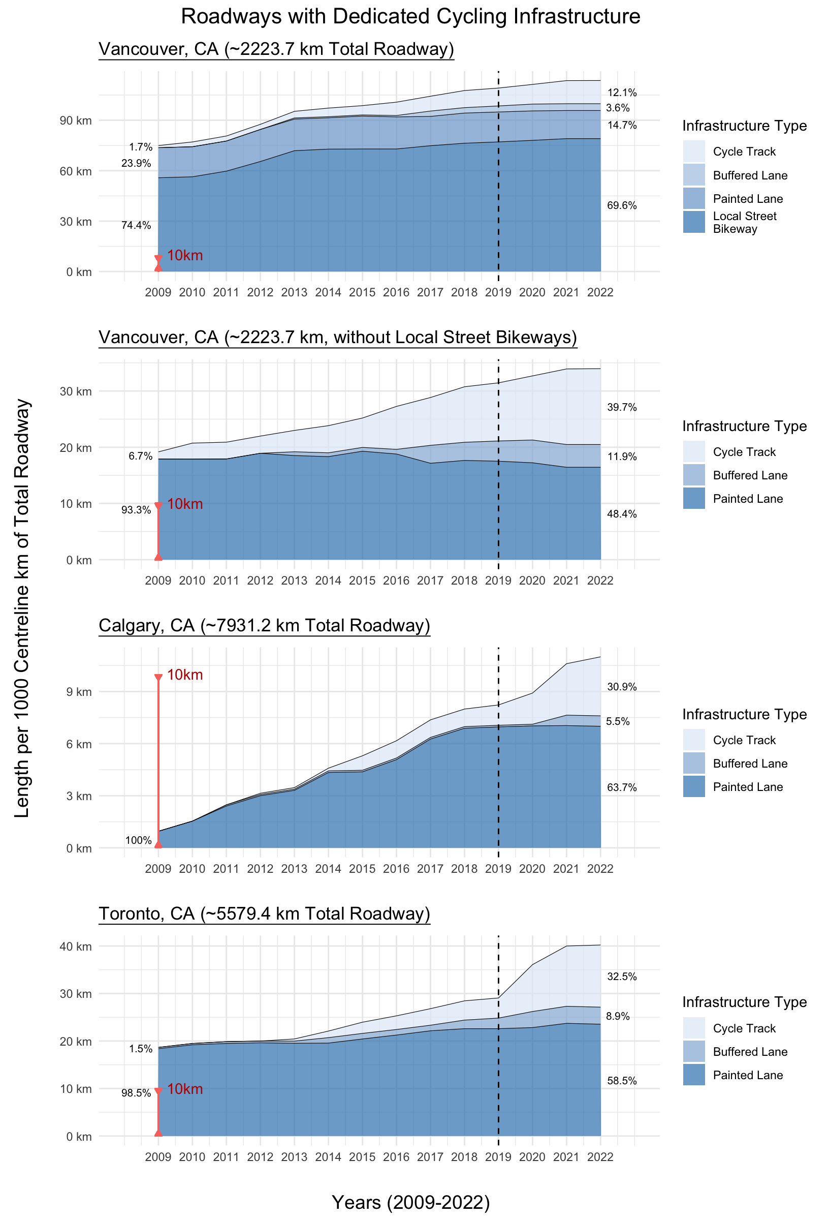
Figure 3b: A comparative analysis between municipal data and verified data on the installation years for cycling infrastructure in Calgary, CA.
# Create the plot
sfig8 <- plot_yearly_diff(
calg,
x_lim = c(-10, 21),
title = "Difference in Installation Years, Comparing City Data and Verified Data: Calgary, CA",
out_data = TRUE
)
# Calc metrics for description
sfig8_n <- sum(sfig8$data$n)
sfig8_0 <- sfig8$data %>% # perc correct
filter(year_diff == 0) %>%
pull(n_perc) %>%
round(1)
sfig8_pm1 <- sfig8$data %>% # perc plus/minus 1
filter(year_diff >= -1 & year_diff <= 1) %>%
pull(n_perc) %>%
sum %>%
round(1)Any data where a city provided and verified installation years were missing or the verified year occurred earlier or equal to the start of the study period (2009) has been excluded from analysis, yielding n=669 segments. The graph shows that 42.2% of the included segments had the correct installation year as per the city’s data, and 62.8% were accurate within a range of ±1 year.
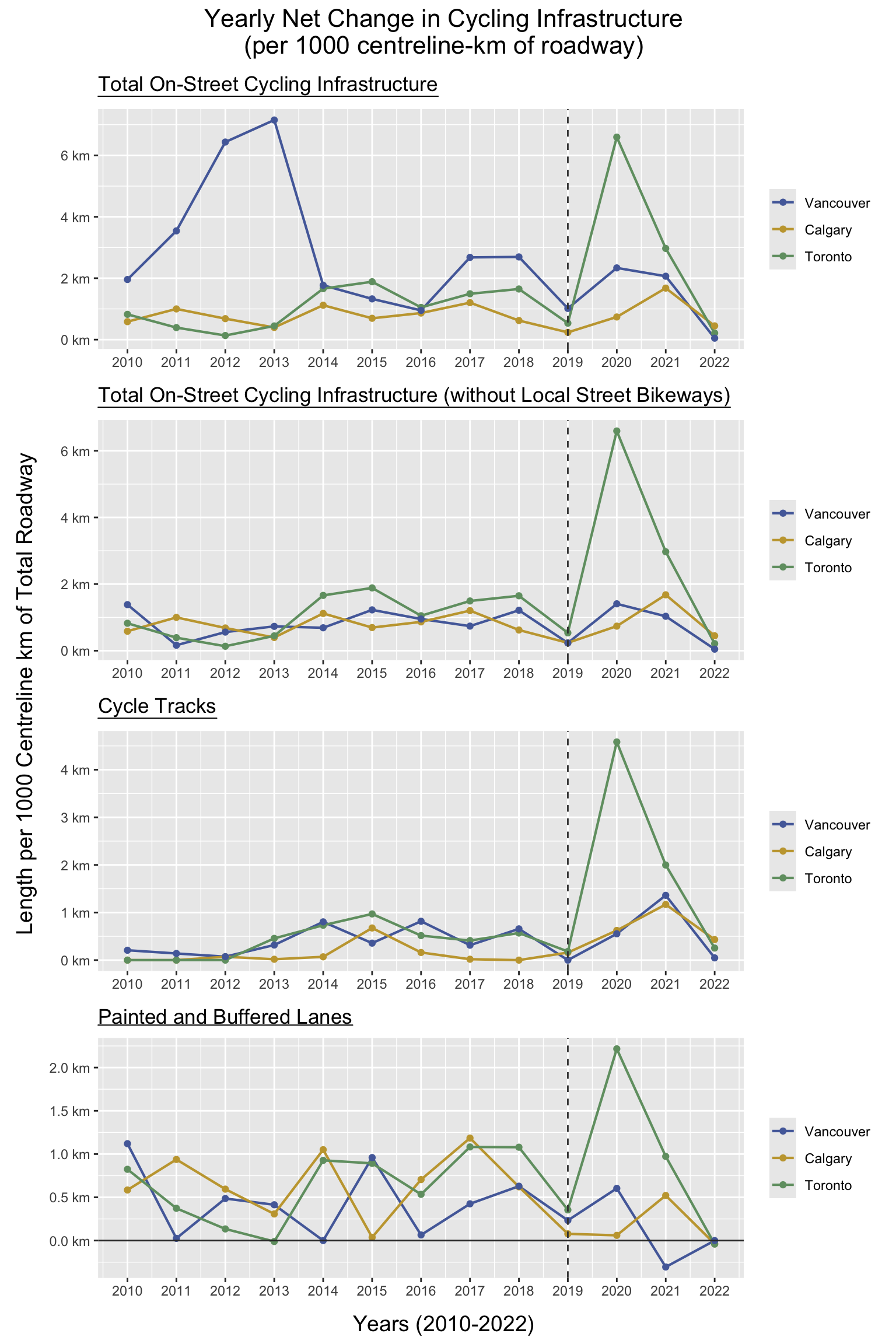
Figure 3c: A comparative analysis between municipal data and verified data on the installation years for cycling infrastructure in Toronto, CA.
# Create the plot
sfig9 <- plot_yearly_diff(
toron,
x_lim = c(-10, 21),
title = "Difference in Installation Years, Comparing City Data and Verified Data: Toronto, CA",
out_data = TRUE
)
# Calc metrics for description
sfig9_n <- sum(sfig9$data$n)
sfig9_0 <- sfig9$data %>% # perc correct
filter(year_diff == 0) %>%
pull(n_perc) %>%
round(1)
sfig9_pm1 <- sfig9$data %>% # perc plus/minus 1
filter(year_diff >= -1 & year_diff <= 1) %>%
pull(n_perc) %>%
sum %>%
round(1)Any data where a city provided and verified installation years were missing or the verified year occurred earlier or equal to the start of the study period (2009) has been excluded from analysis, yielding n=188 segments. The graph shows that 74.5% of the included segments had the correct installation year as per the city’s data, and 78.2% were accurate within a range of ±1 year.
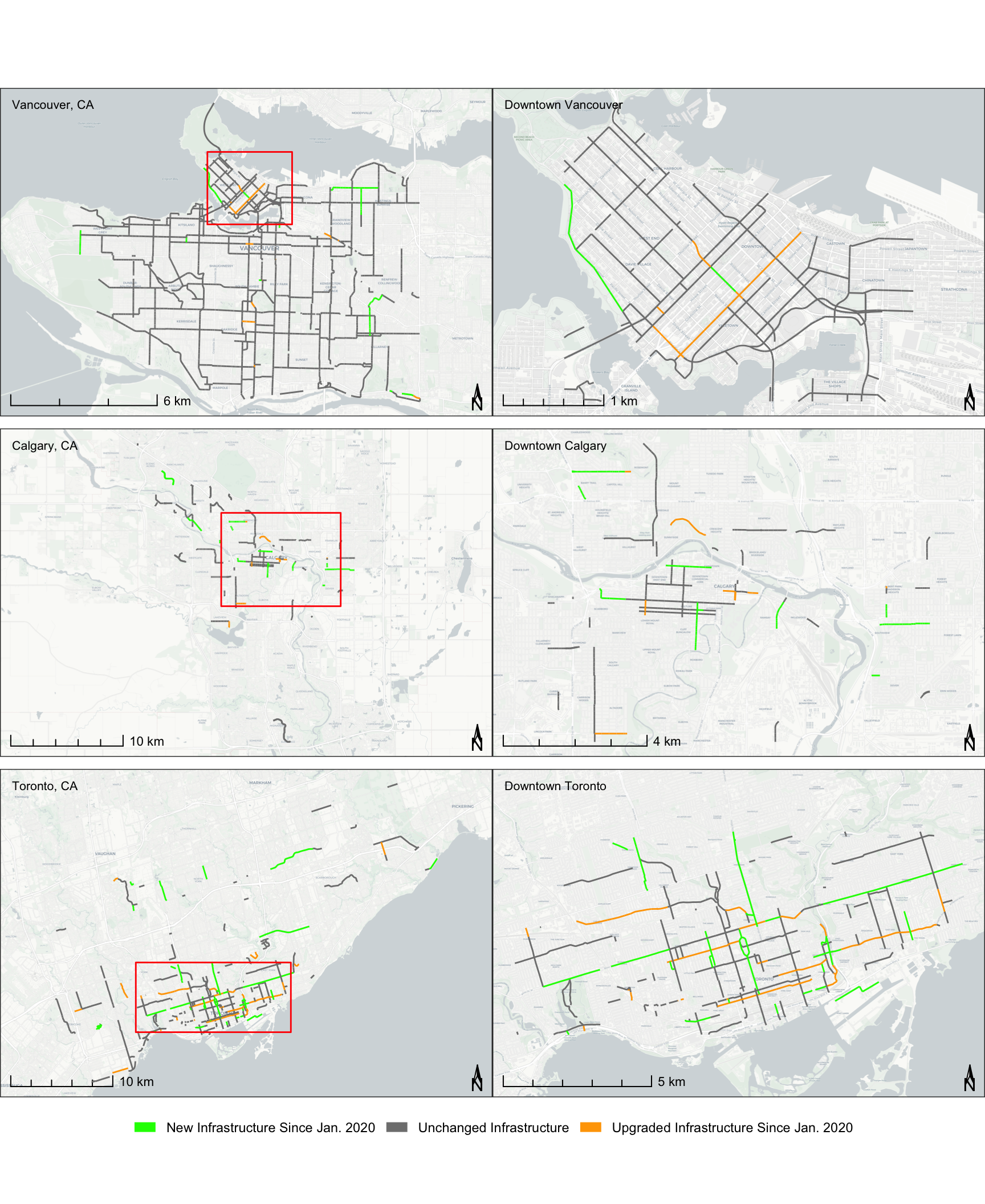
Figure 4: Changes in dedicated cycling infrastructure between 2009 and 2022 for Vancouver, Calgary, and Toronto by infrastructure category.
Assessed using roadway centreline-km, with infrastructure classifications determined by the most protective element present along each road segment.
fig2 <- plot_yearly_len_infra(
df_list = list(
"Vancouver, CA (~2223.7 km Total Roadway)" = list(
data = vanc,
roadway_per = 1000,
roadway_total = 2223.7,
color_manual = c(
"#DFEBF7",
"#bbcbe3",
"#3683BB",
"#256180"
)
),
"Vancouver, CA (~2223.7 km, without Local Street Bikeways)" = list(
data = vanc %>% filter(verify_install_type != "LSB"),
roadway_per = 1000,
roadway_total = 2223.7
),
"Calgary, CA (~7931.2 km Total Roadway)" = list(
data = calg,
roadway_per = 1000,
roadway_total = 7931.2
),
"Toronto, CA (~5579.4 km Total Roadway)" = list(
data = toron,
roadway_per = 1000,
roadway_total = 5579.4
)
),
len_title = "Length per 1000 Centreline km of Total Roadway",
len_per_start = TRUE,
len_per_end = TRUE,
line_km = 10
)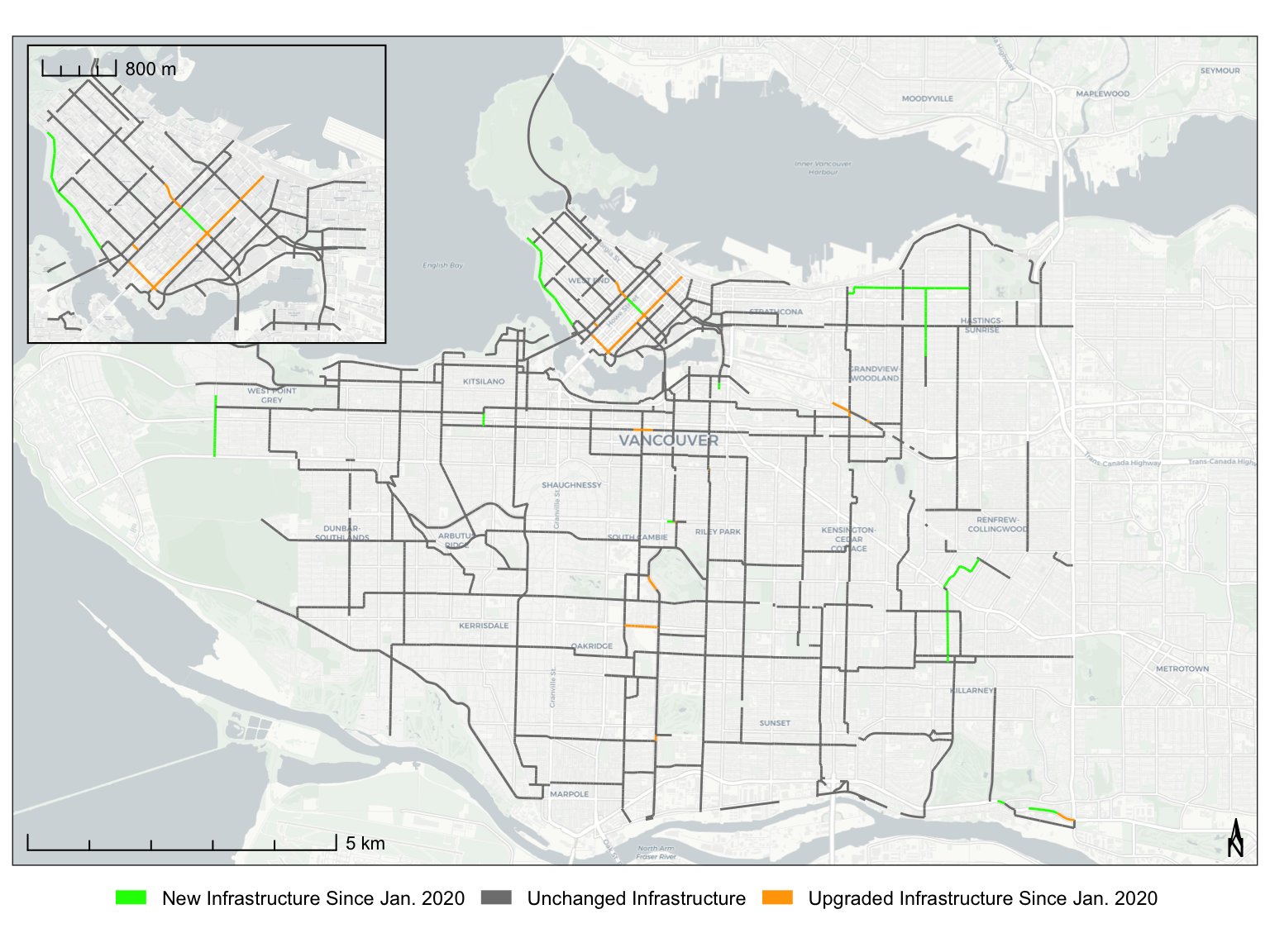
Figure 5: Yearly net change in cycle route infrastructure by municipality, standardized per 1000 centerline-km of roadway.
The net change considers both the installation of new facilities, and the removal of existing infrastructure, such as when an existing facility is upgraded. Cycle route infrastructure is defined by the most protective element along a street centreline. This reflects the overall modifications made within each municipality over the course of the study period (2009-2022).
fig3 <- plot_yearly_change(
df_list = list(
"Vancouver, CA" = list(
city = "Vancouver",
data = vanc,
roadway_per = 1000,
roadway_total = 2223.7
),
"Calgary, CA" = list(
city = "Calgary",
data = calg,
roadway_per = 1000,
roadway_total = 7931.2
),
"Toronto, CA" = list(
city = "Toronto",
data = toron,
roadway_per = 1000,
roadway_total = 5579.4
)
),
len_title = "Length per 1000 Centreline km of Total Roadway",
ylims = lapply(1:4, function(x) c(0, 8))
)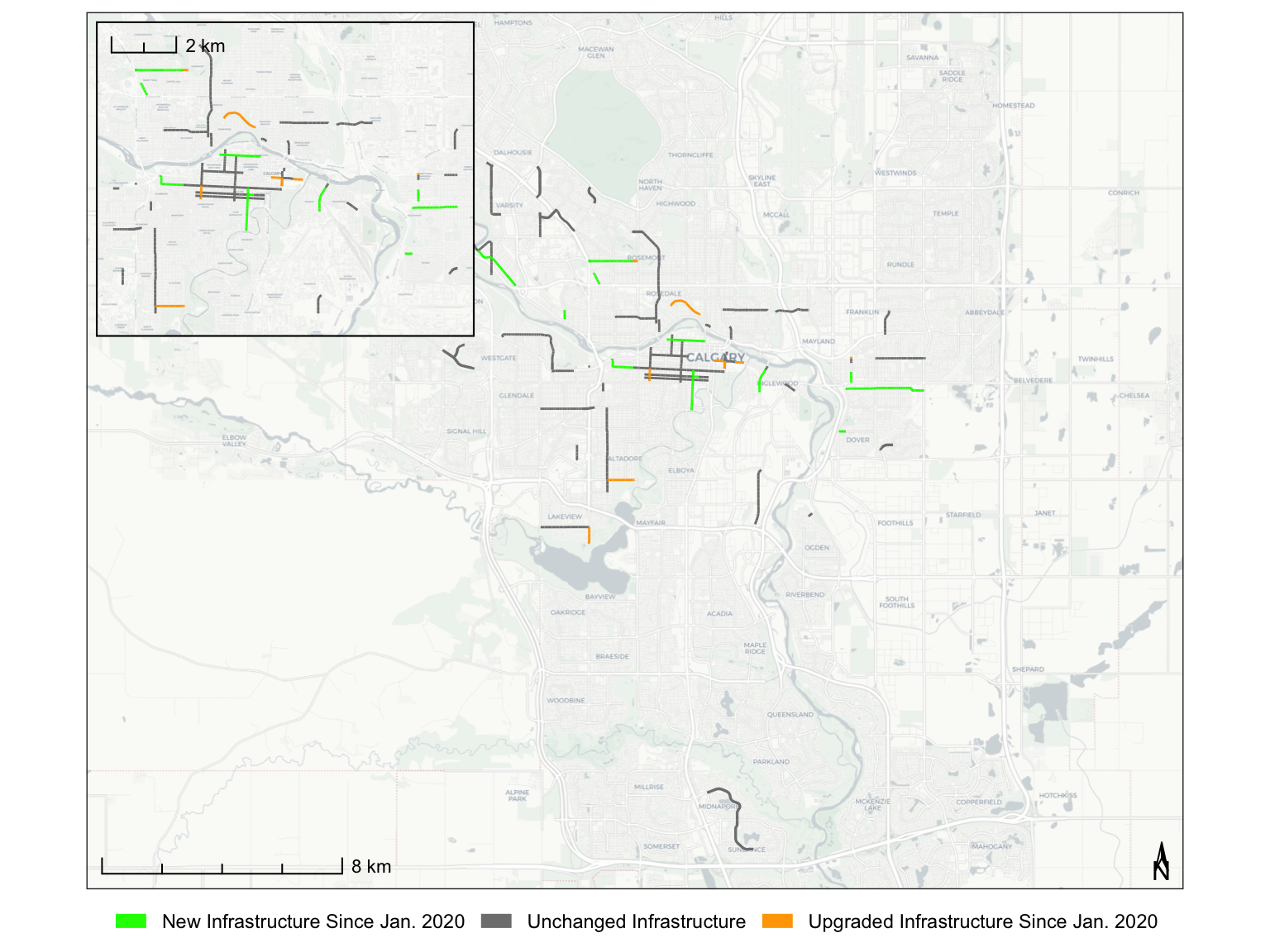
Figure 6a: Changes in dedicated cycling infrastructure between 2009 and 2021 for the Municipality of Vancouver, CA.
By (A) roadway classification, and (B) infrastructure distribution within each road class. Assessed using roadway centreline-km, with infrastructure classification determined by the most protective element present along each road segment.
sfig4 <- list()
sfig4 <- plot_yearly_len_road(
vanc,
title = "Roadways with Dedicated Cycling Infrastructure (Vancouver, CA)"
)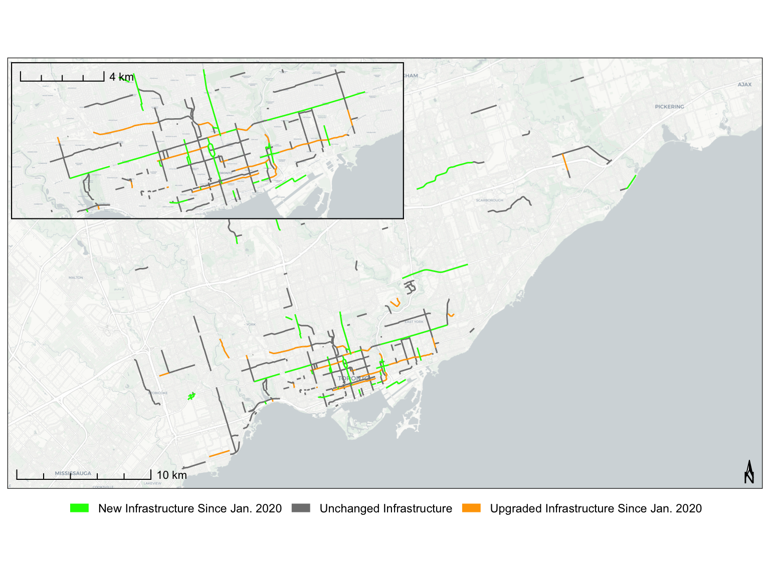
Figure 6b: Changes in dedicated cycling infrastructure between 2009 and 2022 for the Municipality of Calgary, CA.
By (A) roadway classification, and (B) infrastructure distribution within each road class. Assessed using roadway centreline-km, with infrastructure classification determined by the most protective element present along each road segment.
sfig5 <- list()
sfig5 <- plot_yearly_len_road(
calg,
title = "Roadways with Dedicated Cycling Infrastructure (Calgary, CA)"
)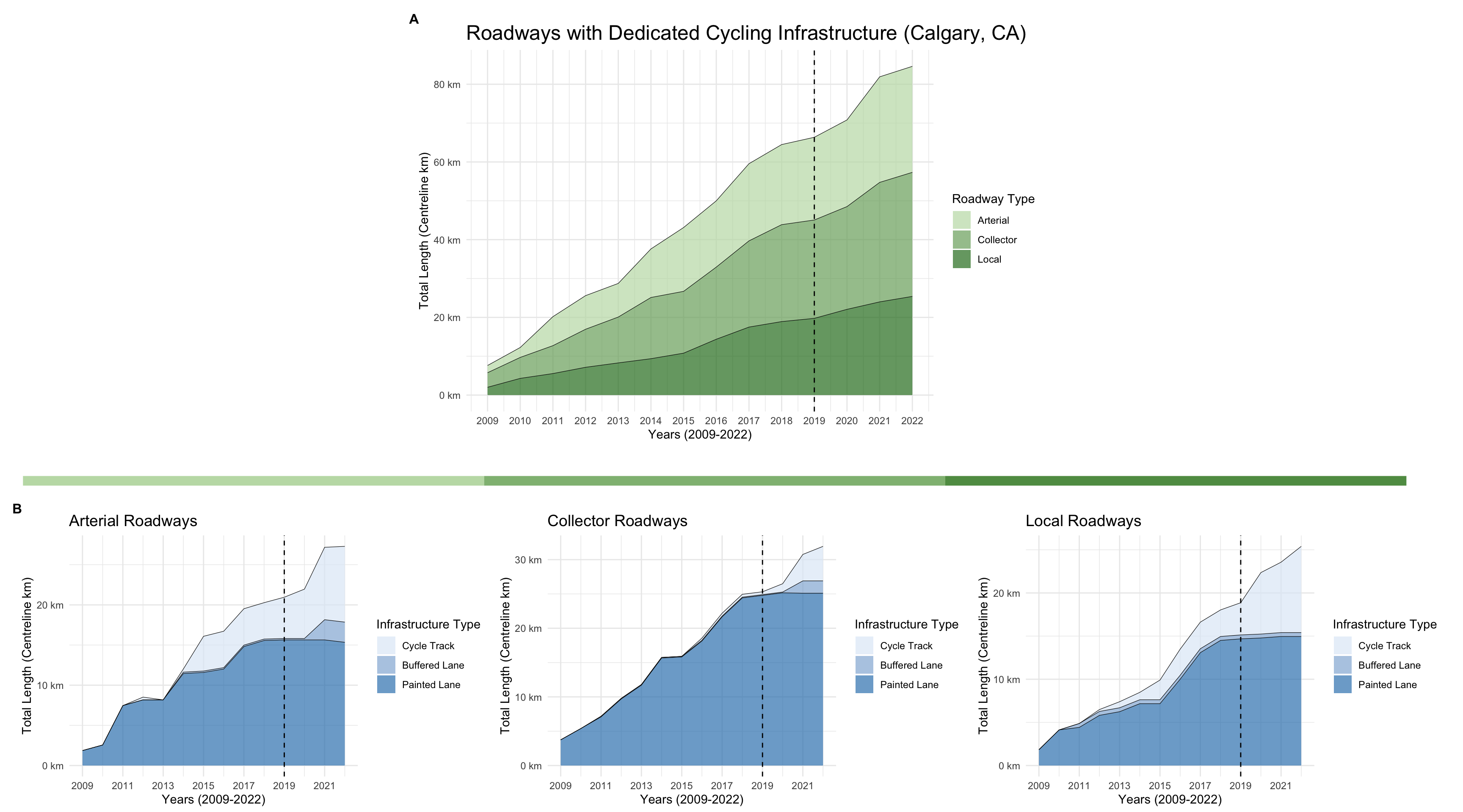
Figure 6c: Changes in dedicated cycling infrastructure between 2009 and 2022 for the Municipality of Toronto, CA.
By (A) roadway classification, and (B) infrastructure distribution within each road class. Assessed using roadway centreline-km, with infrastructure classification determined by the most protective element present along each road segment.
sfig6 <- list()
sfig6 <- plot_yearly_len_road(
toron,
title = "Roadways with Dedicated Cycling Infrastructure (Toronto, CA)"
)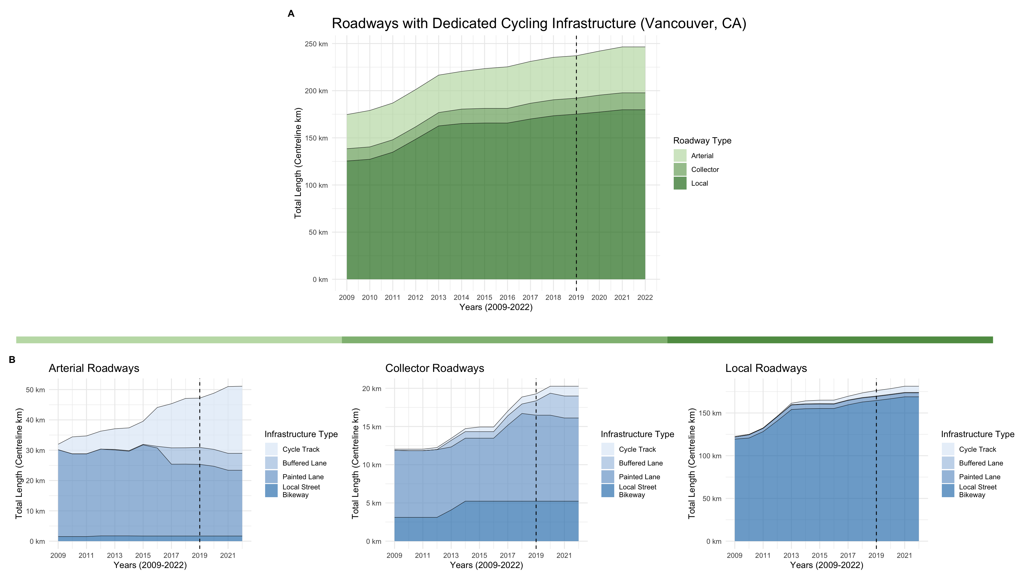


Figure 7: Changes in dedicated on-street infrastructure since January 2020 for Vancouver, Calgary, and Toronto with municipal boundaries.
New installations of dedicated infrastructure are denoted in green, upgrades from a previous dedicated infrastructure type are denoted in orange. Basemap from OpenStreetMap and Carto (Positron).
Figure files available at:

# Save pdf
ggsave(
"../manuscript/figures/fig-maps.pdf",
fig4$plot,
width = 10,
height = 12
)
# Save png
ggsave(
"../manuscript/figures/fig-maps.png",
fig4$plot,
width = 10,
height = 12
)
# Display figure
fig4$plot %>% print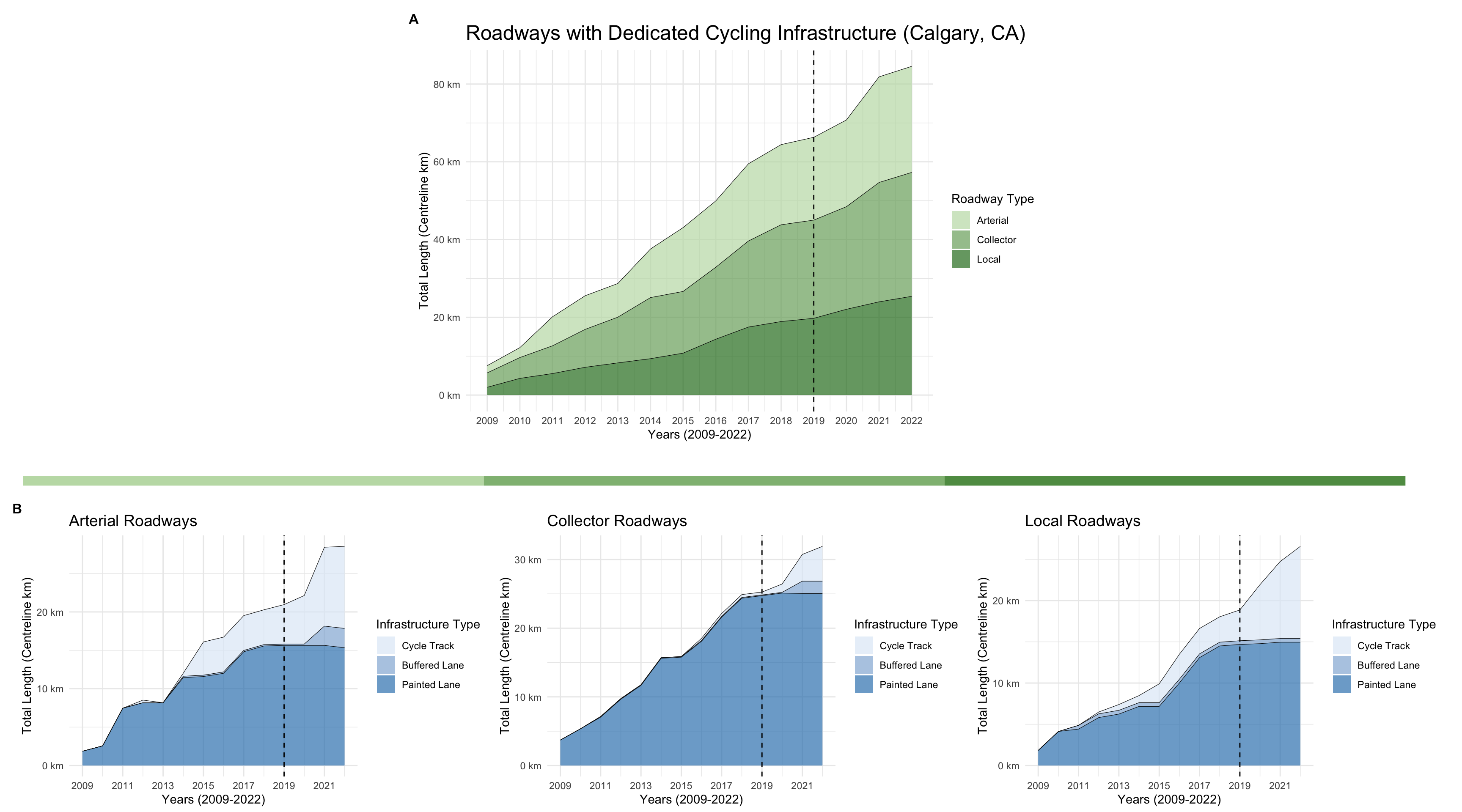
Past Supplementary Results
Past Supplementary Figure 1: Enlarged Map. Changes in Dedicated On-Street Infrastructure Between 2020-2021 for the Municipality of Vancouver, CA.
New installations of dedicated infrastructure are denoted in green, upgrades from a previous dedicated infrastructure type are denoted in orange. Basemap from OpenStreetMap and Carto (Positron).
sfig1 <- list()
sfig1$plot <- map_infra_detail(
map_data,
"vancouver",
map_inset_position = c(
left = -0.9,
bottom = 0.65,
right = 1.2125,
top = 0.99
),
map_ratio = 1.5,
map_inset_ratio = 1.2
)Figure files available at:

# Save pdf
ggsave(
"../manuscript/figures/sfig-map-vanc.pdf",
sfig1$plot,
width = 11
)
# Save png
ggsave(
"../manuscript/figures/sfig-map-vanc.png",
sfig1$plot,
width = 11
)
# Display figure
sfig1$plot %>% print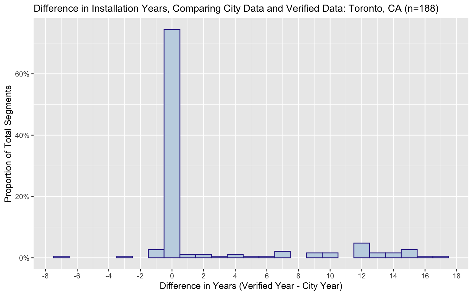
Past Supplementary Figure 2: Enlarged Map. Changes in Dedicated On-Street Infrastructure Between 2020-2022 for the Municipality of Calgary, CA.
New installations of dedicated infrastructure are denoted in green, upgrades of dedicated infrastructure are denoted in orange. Basemap from OpenStreetMap and Carto (Positron).
sfig2 <- list()
sfig2$plot <- map_infra_detail(
map_data,
"calgary",
map_inset_position = c(
left = -0.85,
bottom = 0.65,
right = 1.2125,
top = 0.99
),
map_ratio = 1.25,
map_inset_ratio = 1.2
)Figure files available at:

# Save pdf
ggsave(
"../manuscript/figures/sfig-map-calg.pdf",
sfig2$plot,
width = 11
)
# Save png
ggsave(
"../manuscript/figures/sfig-map-calg.png",
sfig2$plot,
width = 11
)
# Display figure
sfig2$plot %>% print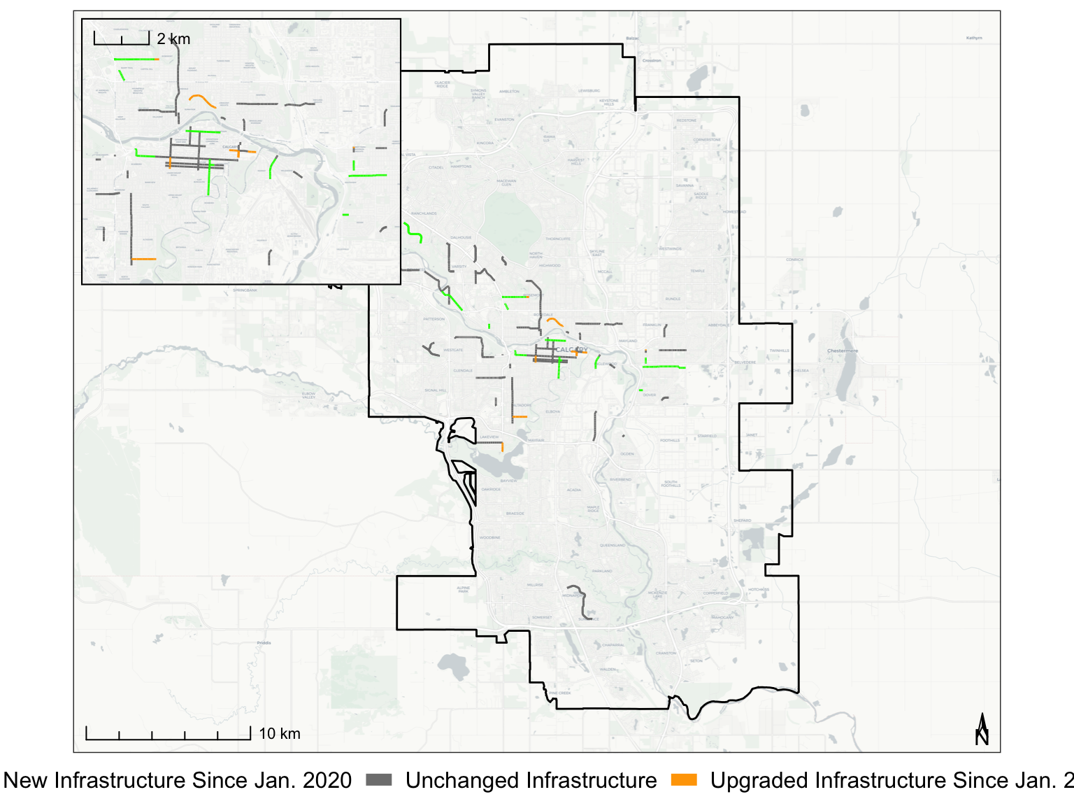
Past Supplementary Figure 3: Enlarged Map. Changes in Dedicated On-Street Infrastructure Between 2020-2022 for the Municipality of Toronto, CA.
New installations of dedicated infrastructure are denoted in green, upgrades of dedicated infrastructure are denoted in orange. Basemap from OpenStreetMap and Carto (Positron).
sfig3 <- list()
sfig3$plot <- map_infra_detail(
map_data,
"toronto",
map_inset_position = c(
left = -0.85,
bottom = 0.65,
right = 1.38,
top = 0.99
),
map_ratio = 1.75,
map_inset_ratio = 2.5
)Figure files available at:

# Save pdf
ggsave(
"../manuscript/figures/sfig-map-toron.pdf",
sfig3$plot,
width = 11
)
# Save png
ggsave(
"../manuscript/figures/sfig-map-toron.png",
sfig3$plot,
width = 11
)
# Display figure
sfig3$plot %>% print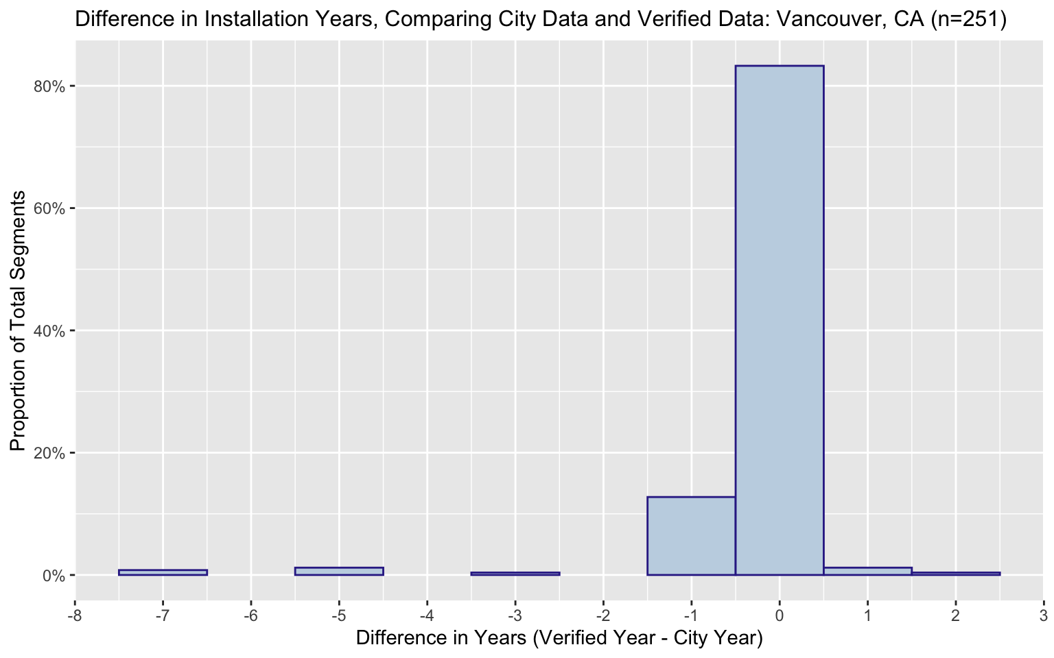
Past Supplementary Table 1: Total Length of Dedicated On-Street Cycling Infrastructure between 2009 and 2022, for Vancouver, Calgary, and Toronto (Canada).
Each entry denotes the aggregated length of infrastructure existing at the conclusion the calendar year. Lengths are measured in roadway centreline-km, with cycling infrastructure classified according to the side of the road featuring the most protective element. Rows noted in light red denote infrastructure changes following the start of the COVID-19 pandemic.
# Setup table list
stab1 <- list()
# Calculated adjusted yearly road lengths for each type
stab1$data <- bind_rows(
calc_yearly_adj_len(vanc) %>% mutate(city = "Vancouver"),
calc_yearly_adj_len(calg) %>% mutate(city = "Calgary"),
calc_yearly_adj_len(toron) %>% mutate(city = "Toronto")
) %>%
pivot_wider( # pivot infra types per col
names_from = type,
values_from = adj_len,
values_fill = 0
) %>%
group_by(year, city) %>%
summarize( # Calculate yearly road len for each type
PL = round(sum(PL, na.rm = TRUE), 2),
BUF = round(sum(BUF, na.rm = TRUE), 2),
CT = round(sum(PBL, na.rm = TRUE), 2)
) %>%
filter(
year >= settings$year_min &
year <= settings$year_max
) %>%
ungroup() %>% mutate( # Calc total road len based on type
TOTAL = PL + BUF + CT
) %>%
group_by(city) %>% arrange(year) %>% mutate(
Change = TOTAL - lag(TOTAL) # change in total road len
) %>%
rename(
Year = year,
City = city
)
# Create side by side tables by city using joins
stab1$data <- stab1$data %>% filter(City == "Vancouver") %>%
select(-City) %>%
left_join(
stab1$data %>% filter(City == "Calgary"),
by = "Year",
suffix = c("_vancouver", "_calgary")
) %>%
left_join(
stab1$data %>% filter(City == "Toronto") %>% rename_with(~ paste0(.x, "_toronto")),
by = join_by(Year == Year_toronto)
) %>%
select(
-City_vancouver,
-City_calgary,
-City_toronto
)
# Gen table
options(knitr.kable.NA = "")
stab1$table <- stab1$data %>%
kable(
col.names = gsub("\\_vancouver|\\_calgary|\\.toronto", "", names(.)),
booktabs = T
) %>%
kable_classic() %>%
column_spec(
c(5,6, 10, 11, 15, 16),
background = "grey90"
) %>%
row_spec(
0,
bold = T
) %>%
row_spec(
12:14,
background = "grey70"
) %>%
add_header_above(
c(" " = 1, "Vancouver" = 5, "Calgary" = 5, "Toronto" = 5),
align = "left"
) %>%
add_header_above(
c(" " = 1, "Measured by centreline-km of roadway" = 15),
italic = T,
bold = F,
align = "left"
) %>%
add_header_above(
c(" " = 1, "Total Length of Roadways with Dedicated Cycling Infrastructure by Year (2009-2022)" = 15),
align = "left",
line = F
)Table
Table files available at:

# Save pdf
if (!file.exists("../manuscript/figures/tab-yearly-len.pdf")) {
save_kable(stab1$table, "../manuscript/figures/tab-yearly-len.pdf")
}
# Save png
if (!file.exists("../manuscript/figures/tab-yearly-len.png")) {
save_kable(stab1$table, "../manuscript/figures/tab-yearly-len.png", zoom = 2)
}
# Display table
stab1$table|
Total Length of Roadways with Dedicated Cycling Infrastructure by Year
(2009-2022)
|
|||||||||||||||
|---|---|---|---|---|---|---|---|---|---|---|---|---|---|---|---|
|
Measured by centreline-km of roadway
|
|||||||||||||||
|
Vancouver
|
Calgary
|
Toronto
|
|||||||||||||
| Year | PL | BUF | CT | TOTAL | Change | PL | BUF | CT | TOTAL | Change | PL_toronto | BUF_toronto | CT_toronto | TOTAL_toronto | Change_toronto |
| 2009 | 39.80 | 0.00 | 2.84 | 42.64 | 7.62 | 0.00 | 0.00 | 7.62 | 102.57 | 1.56 | 0.00 | 104.13 | |||
| 2010 | 39.26 | 0.00 | 6.33 | 45.59 | 2.95 | 12.26 | 0.00 | 0.00 | 12.26 | 4.64 | 107.17 | 1.56 | 0.00 | 108.73 | 4.60 |
| 2011 | 39.32 | 0.00 | 6.64 | 45.96 | 0.37 | 19.15 | 0.55 | 0.00 | 19.70 | 7.44 | 108.72 | 1.56 | 0.00 | 110.28 | 1.55 |
| 2012 | 41.51 | 0.00 | 6.80 | 48.31 | 2.35 | 23.86 | 0.55 | 0.56 | 24.97 | 5.27 | 109.47 | 1.56 | 0.00 | 111.03 | 0.75 |
| 2013 | 39.43 | 1.50 | 8.59 | 49.52 | 1.21 | 26.30 | 0.55 | 0.70 | 27.55 | 2.58 | 108.95 | 2.01 | 2.55 | 113.51 | 2.48 |
| 2014 | 39.01 | 1.50 | 11.20 | 51.71 | 2.19 | 34.45 | 0.73 | 1.25 | 36.43 | 8.88 | 109.13 | 5.89 | 7.75 | 122.77 | 9.26 |
| 2015 | 41.14 | 1.50 | 12.13 | 54.77 | 3.06 | 34.75 | 0.73 | 6.61 | 42.09 | 5.66 | 112.61 | 6.02 | 13.16 | 131.79 | 9.02 |
| 2016 | 40.03 | 1.85 | 17.29 | 59.17 | 4.40 | 40.33 | 0.74 | 7.88 | 48.95 | 6.86 | 115.59 | 6.02 | 16.03 | 137.64 | 5.85 |
| 2017 | 36.38 | 7.09 | 17.97 | 61.44 | 2.27 | 49.73 | 0.74 | 8.03 | 58.50 | 9.55 | 120.02 | 5.50 | 19.97 | 145.49 | 7.85 |
| 2018 | 35.85 | 7.18 | 20.85 | 63.88 | 2.44 | 54.66 | 0.74 | 8.03 | 63.43 | 4.93 | 121.77 | 9.03 | 22.05 | 152.85 | 7.36 |
| 2019 | 35.03 | 8.00 | 21.89 | 64.92 | 1.04 | 55.28 | 0.74 | 9.28 | 65.30 | 1.87 | 121.39 | 11.40 | 23.06 | 155.85 | 3.00 |
| 2020 | 34.32 | 9.00 | 23.86 | 67.18 | 2.26 | 55.76 | 0.74 | 14.48 | 70.98 | 5.68 | 118.82 | 16.34 | 51.89 | 187.05 | 31.20 |
| 2021 | 32.55 | 9.00 | 28.25 | 69.80 | 2.62 | 55.87 | 4.76 | 21.04 | 81.67 | 10.69 | 123.78 | 12.23 | 67.06 | 203.07 | 16.02 |
| 2022 | 33.05 | 9.00 | 28.25 | 70.30 | 0.50 | 55.58 | 4.76 | 24.47 | 84.81 | 3.14 | 122.77 | 12.23 | 69.26 | 204.26 | 1.19 |
Appendix 2 - Methodology
Past Supplementary Table 2: Excluded Segment Types for Vancouver, Calgary, and Toronto (Canada).
# Setup table list
stab2 <- list()
# Get excluded segments for each city
stab2$df <- vanc_preprocess %>%
filter(!id %in% vanc$id) %>%
select(install_type, road_type) %>%
mutate(city = "vancouver") %>%
add_row(
calg_preprocess %>%
filter(!id %in% calg$id) %>%
select(install_type, road_type) %>%
mutate(city = "calgary")
) %>%
add_row(
toron_preprocess %>%
filter(!id %in% toron$id) %>%
select(install_type, road_type) %>%
mutate(city = "toronto")
) %>%
mutate(install_type = str_to_title(install_type))
# Count excluded segments and calc their lengths
stab2$data <- stab2$df %>%
group_by(city, install_type, road_type) %>%
summarize( # count types and len in km
n = n(),
len_km = (sum(st_length(geometry), na.rm = T) / 1000) %>% as.numeric
) %>%
as_tibble %>%
select(-geometry) %>%
group_by(city) %>%
arrange(desc(len_km), .by_group = T)
# Calculate the total segments and length per type
stab2$data <- stab2$data %>%
rename(
"Type" = install_type,
"Class" = road_type,
Segments = n,
Length = len_km
) %>%
group_by(city) %>%
group_map(~{
.x %>%
add_row(
"Type" = "TOTAL",
"Class" = NA,
"Segments" = sum(.x$Segments, na.rm = T),
"Length" = sum(.x$Length, na.rm = T)
)
}, .keep = T) %>%
reduce(add_row) %>%
rename(
City = city
) %>%
mutate(
City = str_to_title(City)
)
# Created formatted side by side table of cities
options(knitr.kable.NA = "")
stab2$table <- stab2$data %>%
mutate(across(
ends_with("Length"),
~ if_else(!is.na(.x), paste0(round(.x, 1), " km"), NA)
)) %>%
kable(
booktabs = T
) %>%
kable_classic() %>%
add_header_above(
c("Measured by centreline-km of roadway" = 5),
italic = T,
bold = F,
align = "left"
) %>%
add_header_above(
c("Excluded Segment Counts and Lengths by Infrastructure Type and Road Classification" = 5),
align = "left",
bold = T,
line = F
) %>%
column_spec(1, bold = T) %>%
row_spec(0, bold = T) %>%
row_spec(
which(stab2$data$Type == "TOTAL"),
bold = T,
extra_css = "border-bottom: 1px solid; border-top: 1px solid"
) %>%
collapse_rows(columns = 1)Table
Table files available at:

# Save pdf
if (!file.exists("../manuscript/figures/tab-excl-infra.pdf")) {
save_kable(stab2$table, "../manuscript/figures/tab-excl-infra.pdf")
}
# Save png
if (!file.exists("../manuscript/figures/tab-excl-infra.png")) {
save_kable(stab2$table, "../manuscript/figures/tab-excl-infra.png", zoom = 2)
}
# Display table
stab2$table|
Excluded Segment Counts and Lengths by Infrastructure Type and Road
Classification
|
||||
|---|---|---|---|---|
|
Measured by centreline-km of roadway
|
||||
| City | Type | Class | Segments | Length |
| Calgary | On-Street Bikeway | 2889 | 437.4 km | |
| Neighbourhood Greenway | 358 | 23.8 km | ||
| Shared Lane | 115 | 18.7 km | ||
| Decommissioned | 3 | 2.8 km | ||
| Cycle Track | 30 | 2.4 km | ||
| Bicycle Lane | 14 | 0.6 km | ||
| Temporary | 6 | 0.5 km | ||
| Cycle Track | Neighbourhood Boulevard | 2 | 0.5 km | |
| On-Street Bikeway | Collector | 1 | 0 km | |
| On-Street Bikeway | Arterial Street | 1 | 0 km | |
| TOTAL | 3419 | 486.7 km | ||
| Toronto | Multi-Use Trail | 330 | 289.3 km | |
| Signed Route (No Pavement Markings) | 215 | 100 km | ||
| Multi-Use Trail - Boulevard | 44 | 37.9 km | ||
| Sharrows - Wayfinding | 97 | 37.4 km | ||
| Multi-Use Trail - Entrance | 179 | 26.2 km | ||
| Park Road | 34 | 22 km | ||
| Sharrows | 55 | 21.5 km | ||
| Multi-Use Trail - Existing Connector | 18 | 9.5 km | ||
| Sharrows - Arterial - Connector | 10 | 3.3 km | ||
| Multi-Use Trail - Connector | 10 | 2.7 km | ||
| Bike Lane | Major Arterial | 2 | 0.6 km | |
| Bike Lane - Contraflow | Local | 1 | 0.2 km | |
| Bike Lane | Minor Arterial | 1 | 0.1 km | |
| Bi-Directional Cycle Track | Local | 1 | 0.1 km | |
| TOTAL | 997 | 550.8 km | ||
| Vancouver | Protected Bike Lanes | Off-street | 317 | 72.7 km |
| Shared Lanes | Arterial | 109 | 8.7 km | |
| Shared Lanes | Residential | 11 | 3.1 km | |
| Shared Lanes | Collector | 36 | 2.8 km | |
| Shared Lanes | Sec Arterial | 38 | 2.6 km | |
| Protected Bike Lanes | Lane | 8 | 1.4 km | |
| Protected Bike Lanes | Arterial | 8 | 1.3 km | |
| Protected Bike Lanes | Residential | 12 | 0.7 km | |
| Painted Lanes | Arterial | 2 | 0.6 km | |
| Protected Bike Lanes | Sec Arterial | 2 | 0.4 km | |
| Painted Lanes | Residential | 2 | 0.2 km | |
| Painted Lanes | Lane | 1 | 0.1 km | |
| Painted Lanes | Sec Arterial | 1 | 0.1 km | |
| Local Street | Off-street | 1 | 0.1 km | |
| Local Street | Residential | 1 | 0 km | |
| TOTAL | 549 | 94.7 km | ||
Contributions
Richard Wen developed reproducible R code and organized the data based on Konrad Samsel’s draft manuscript and previous R code. Konrad Samsel prepared draft manuscript, raw data, and provided consultation on data and methods.
Acknowledgements
Linda Rothman and Brice Batomen provided supervision, project administration, resources, funding, and review/editing for the draft manuscript.
Software and Package Versions
R and R package versions:
## R version 4.3.3 (2024-02-29)
## Platform: x86_64-apple-darwin20 (64-bit)
## Running under: macOS 15.6.1
##
## Matrix products: default
## BLAS: /Library/Frameworks/R.framework/Versions/4.3-x86_64/Resources/lib/libRblas.0.dylib
## LAPACK: /Library/Frameworks/R.framework/Versions/4.3-x86_64/Resources/lib/libRlapack.dylib; LAPACK version 3.11.0
##
## locale:
## [1] en_US.UTF-8/en_US.UTF-8/en_US.UTF-8/C/en_US.UTF-8/en_US.UTF-8
##
## time zone: America/Toronto
## tzcode source: internal
##
## attached base packages:
## [1] stats graphics grDevices utils datasets methods base
##
## other attached packages:
## [1] R.devices_2.17.2 boot_1.3-29 binom_1.1-1.1 DT_0.33
## [5] kableExtra_1.4.0 units_0.8-5 prettymapr_0.2.5 ggspatial_1.1.9
## [9] tmap_3.3-4 sf_1.0-21 rsvg_2.6.0 magick_2.8.3
## [13] webshot2_0.1.1 DiagrammeRsvg_0.1 DiagrammeR_1.0.11 patchwork_1.2.0
## [17] scales_1.3.0 ggtext_0.1.2 readxl_1.4.3 glue_1.7.0
## [21] lubridate_1.9.3 forcats_1.0.0 stringr_1.5.1 dplyr_1.1.2
## [25] purrr_1.0.1 readr_2.1.4 tidyr_1.3.0 tibble_3.2.1
## [29] ggplot2_3.5.2 tidyverse_2.0.0 knitr_1.43 bookdown_0.38
## [33] rmarkdown_2.26
##
## loaded via a namespace (and not attached):
## [1] RColorBrewer_1.1-3 rstudioapi_0.15.0 jsonlite_1.8.8
## [4] wk_0.9.1 magrittr_2.0.3 farver_2.1.1
## [7] vctrs_0.6.5 base64enc_0.1-3 terra_1.7-71
## [10] htmltools_0.5.7 leafsync_0.1.0 curl_5.2.1
## [13] raster_3.6-26 cellranger_1.1.0 s2_1.1.6
## [16] sass_0.4.7 KernSmooth_2.23-22 bslib_0.5.0
## [19] htmlwidgets_1.6.4 plyr_1.8.9 stars_0.6-4
## [22] cachem_1.0.8 lifecycle_1.0.4 pkgconfig_2.0.3
## [25] R6_2.5.1 fastmap_1.1.1 digest_0.6.33
## [28] colorspace_2.1-0 ps_1.7.5 leafem_0.2.3
## [31] rosm_0.3.0 crosstalk_1.2.1 lwgeom_0.2-14
## [34] labeling_0.4.3 fansi_1.0.6 timechange_0.3.0
## [37] abind_1.4-5 compiler_4.3.3 proxy_0.4-27
## [40] bit64_4.0.5 withr_3.0.0 DBI_1.2.2
## [43] highr_0.10 R.utils_2.12.3 tmaptools_3.1-1
## [46] leaflet_2.2.2 classInt_0.4-10 tools_4.3.3
## [49] chromote_0.2.0 R.oo_1.25.0 promises_1.2.1
## [52] gridtext_0.1.5 grid_4.3.3 generics_0.1.3
## [55] gtable_0.3.4 leaflet.providers_2.0.0 tzdb_0.4.0
## [58] R.methodsS3_1.8.2 class_7.3-22 websocket_1.4.1
## [61] hms_1.1.3 sp_2.1-3 xml2_1.3.6
## [64] utf8_1.2.4 pillar_1.9.0 vroom_1.6.3
## [67] later_1.3.1 lattice_0.22-5 bit_4.0.5
## [70] tidyselect_1.2.0 V8_4.4.2 svglite_2.1.3
## [73] xfun_0.42 visNetwork_2.1.2 stringi_1.8.3
## [76] yaml_2.3.7 evaluate_0.21 codetools_0.2-19
## [79] cli_3.6.2 systemfonts_1.0.4 munsell_0.5.0
## [82] processx_3.8.2 jquerylib_0.1.4 dichromat_2.0-0.1
## [85] Rcpp_1.0.12 png_0.1-8 XML_3.99-0.16.1
## [88] parallel_4.3.3 ellipsis_0.3.2 viridisLite_0.4.2
## [91] e1071_1.7-14 crayon_1.5.2 rlang_1.1.3RStudio version:
## $citation
## To cite RStudio in publications use:
##
## Posit team (2026). RStudio: Integrated Development Environment for R.
## Posit Software, PBC, Boston, MA. URL http://www.posit.co/.
##
## A BibTeX entry for LaTeX users is
##
## @Manual{,
## title = {RStudio: Integrated Development Environment for R},
## author = {{Posit team}},
## organization = {Posit Software, PBC},
## address = {Boston, MA},
## year = {2026},
## url = {http://www.posit.co/},
## }
##
## $mode
## [1] "desktop"
##
## $version
## [1] '2026.1.2.418'
##
## $long_version
## [1] "2026.01.2+418"
##
## $release_name
## [1] "Apple Blossom"